12.3 Anatomy of an exponential function

Julian Pakay

12.3 Anatomy of an exponential function

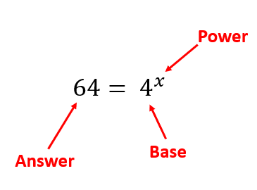
One confusing aspect in all this is that exponential functions may look similar to functions like y = x². But they are quite different in that the variable x is instead in the superscript position (i.e. is the exponent). For example, in y=4^x, the variable x is the exponent, and 4 is a constant and the base. The difficulty in making predictions based on exponential functions is often due to having to solve for an unknown exponent.

Why is Euler’s number so important?

Euler’s number, usually just shown as e, is a very important number in mathematics and appears in many functions that describe natural phenomena. It is worth understanding its origins. e is approximated by 2.718 but is an irrational number (i.e. it cannot be written as a simple fraction) and the base of the natural logarithms. e was discovered by Swiss mathematician Leonhard Euler (1707–1783), who was investigating compound interest. Compound interest is where interest earnt on money is added to the principal and interest earnt in the next increment is calculated on this compounded amount.

Imagine you deposit $1 in the bank at an annual interest rate of 2%, compounded each year. After five years the interest earnt would be equal to:

$\displaystyle $(1 + 0.02) ^{5}$

If this interest was instead calculated and compounded each quarter, it would be equal to:

$\displaystyle $(1 + 0.02/4)^{4 \times 5}$

You can see that you will earn more money if the interest is calculated and compounded with more increments. But as you increase the number of increments does the amount increase indefinitely? You could describe this by a more general equation:

$\displaystyle \$ \underset {n \rightarrow \infty}{\text{lim}} (1 + 1/n)^{n}$

The answer here is no. As you increase the number of increments (n), the total will start to converge on the value of e (2.718).This equation for compound interest also appears when modelling many natural processes – you can think of population growth as similar to compound interest.

Euler’s number

Euler’s number e becomes very useful where we need to model a relationship in which a constant change in the independent variable gives the same proportional change (i.e. percentage increase or decrease) in the dependent variable. For example, because the growth rate of a population of cells in vitro is proportional to the size of the population then the number of cells at any given time can be modelled by an exponential function such as:

$\displaystyle y = Ae^{bx}$

where

y = the total number of cells at time x

A = the initial number of cells

e = Euler’s number

b = the growth constant

x = time.

e and the natural logarithm

So, e is used in ‘natural’ exponential functions, as the following chart shows.

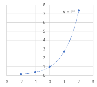
A plot of y = ex, showing that the slope of the curve at any point is equal to the value of ex — Figure 12.3: A plot of y = e^x. The slope of the curve e^x at any point is equal to the value of e^x. This property of e makes it useful for problems related to growth or decay, where the rate of change is determined by the present value of the number being measured.

One of the amazing things about this function of e is that the slope of the line is equal to the value. That is, if you calculate the slope of the curve e^x at any point it is equal to the value of e^x.

So, when x = 0, the value of e^x = 1, and the slope = 1

And when x = 1, the value of e^x = e, and the slope = e

These are important rules to remember when solving exponential functions.

So, a function like e^x is all about describing growth and is useful for determining the amount of growth or total number of things after x units of time.

The natural logarithm is the inverse of e^x. Because of the inverse nature of logarithms, they are very useful for determining the value of an unknown exponent. For example, they allow us to insert the amount of growth into an equation and then work out the amount of time it would take to get there.

What are logarithms?

The simplest way to explain logarithms is that they are functions which allow us to determine how many of a number we need to multiply to get another number. For example, how many 4s do you need to multiply to get 64? 4 × 4 × 4 = 64, so the answer in this case is 3. So, the logarithm is 3. This is written as log₄(64) = 3.

4 × 4 × 4 = 64 or 4³ = 64 is the equivalent of log₄(64) = 3

In this function, 4 is the base of the logarithm. It is the same as the base of the equivalent exponential function.

For the natural logarithm the base is e. It is most often written in the form ln rather than log_e and represents how many times e needs to be multiplied to achieve the desired number. For example:

ln (20.086) = log_e (20.086) ≈ 3, since 2.71828³ ≈ 20.086

A logarithm with base 10 is also known as the common logarithm log₁₀(x) and is most often written as log(x). So, if a log is used and the base is not specified it is safe to assume the base is 10. The common logarithm is used frequently in science and engineering.

log₁₀10 = 1, log₁₀100 = 2, log₁₀1,000 = 3, log₁₀10,000 = 4 and so on.

Working with exponents

In order to solve problems involving exponential functions it is worth examining their properties. These properties will provide you with some easy tools for simplifying exponential equations.

Multiplying like bases

When multiplying exponents with like bases we can simply add the bases. For example:

$\displaystyle x^{2}.x^{3}$

is the equivalent of

$\displaystyle x^{2}.x^{3} = x.x.x.x.x$

$\displaystyle x.x.x.x.x = x^{5}$

which leads to general rule of

$\displaystyle x^{m}.x^{n} = x^{m + n}$

Dividing like bases

Dividing like bases is similar to multiplying like bases except instead of adding the exponents you subtract them. For example:

$\displaystyle \frac {y^{5}}{y^{2}} = \frac {y.y.y.y.y}{y.y} = \frac {y.y.y}{1} = y^{3}$

which leads to general rule of

$\displaystyle y^{m} ÷ y^{n} = y^{m-n}$

Negative powers

Negative exponents may initially seem more difficult to understand. However, a negative exponent just indicates how many times to divide by the base number. For example:

$\displaystyle 4^{-3} = 1/4^{3} = 1 ÷ (4 \times 4 \times 4) = 0.015625$

This means that one way of handling negative exponents is to take the reciprocal of the exponent. When you do this, you change the sign of the exponent from minus to plus or from plus to minus, which leads to general rule of:

$\displaystyle y^{-p} = \frac {1}{y^{p}}$

Zero powers

Any number raised to the power of zero is equal to 1. How does this work? Remember the rule about subtracting the exponents when dividing like bases:

$\displaystyle \frac {y^{3}}{y^{3}} = \frac {y.y.y}{y.y.y} = \frac {1}{1}$

which leads to general rule of

$\displaystyle y^{0} = 1$

Working with logs

An important property of logarithms and exponents is that they are the inverse of one another. That is, if you apply the log to a number and then apply the exponent, providing you use the same base you will get back to the same number. This property can be written as:

$\displaystyle \log_{y}(y^{x}) = x$

and the inverse is

$y^{\log_{y}(x)} = x$

This property can be important for solving exponential functions. For example:

What is x in log₄(x) = 5?

Take the exponent of both sides to determine x:

$4^{\log_{4}(x)} = 4^{5}$

Since $4^{\log_{4}(x)} = x$

then $x = 4^{5} = 1,024$

This leads to the general rule that the log equation can be transformed into its exponential equivalent in this way:

$\displaystyle \log_{b} (M) = N \leftrightarrows M = b^{N}$

This also means that the natural log of e is equal to 1:

ln (e) = 1

Following on from this we get the following properties of logarithms:

$\log_{3} abc$

$= \log_{3} a + \log_{3} b + \log_{3} ac$

and

$\log_{2} \frac {x}{y} = \log_{2}x - \log_{2}y$

This then leads to another important property, which is useful for solving for unknown exponents.

$\log_{c} x^{3}$

$= \log_{c} x.x.x$

$= \log_{c} x + \log_{c} x + \log_{c} x$

$= 3\log_{c} x$

This further leads to a very important general rule:

$\log_{c}x^{n} = n \log_{c} x$

A useful way to further understand logarithms is to use the analogy of growth over time.

If we imagine a population growing over time then the equation $\ln (y) = x$ could be thought of as, how long $(x)$ would it take to get a growth $(y)$ in the population?

If you have the equation $\ln (1) = x$ , then $x$ must be equal to 0.

That is, it takes zero time to reach 1 times the current population.

Therefore, the logarithm of 1 always equals 0.

This also makes sense for logarithms of fractional values.

$\ln (0.5) = x$ could be thought of as, how long $(x)$ would it take to get half the current amount in the population?

To get less than we started with means we must go in reverse.

So, $\ln (0.5) = -0.693$

In terms of time, it would take negative time to have half our current value.

Can you take the logarithm of a negative number? For example:

$\ln (-1) = x$

Using the population growth analogy, the question would be how long would it take to get a negative population? You can’t have a negative population, so the answer is undefined.

Therefore, $\log (\text{anynegativenumber}) = \text{undefined}$

Putting exponents and logs to use

Can we put these properties of logarithms and exponents to use in solving real-world problems?

A strain of E. coli bacteria has a doubling rate of 20 minutes in LB broth at 37 °C. If there are 1,000 E. coli bacteria that are allowed to grow under ideal conditions, how long will it take to reach 1 million bacteria?

We first need to think about how fast the bacteria are growing.

At time zero there are 1,000 bacteria and there is a doubling every 20 minutes (3 times per hour).

Time (minutes)	0	20	40	60	80	120
# Bacteria	1,000	2,000	4,000	8,000	16,000	32,000

This is an exponential rate of growth where the amount of growth in the bacterial population is directly proportional to the size of the population. The first thing to do is define an exponential equation which describes this rate of growth.

Recall the general form of the exponential growth equation:

$y = Ae^{bx}$

where

$y$ = the total number of cells at time x

A = the initial number of cells

e = Euler’s number

b = the growth constant

x = time.

In this case, however, we can be more defined:

$B = (1,000)2^{3t}$

where

$B$ = number of bacteria

1,000 = starting number of bacteria (multiplied by 2 since they double)

t = time (hours) (multiplied by 3 since they double 3 times per hour).

You can check if the equation works by looking at the table of bacterial growth above.

So, when does the number of bacteria equal 1 million?

$1,000,000 =(1,000)2^{3t}$

What we need to do is isolate the exponent t, to be able to solve it. First simplify the equation by dividing both sides by 1,000.

$\frac {1,000,000}{1,000} = \frac {(1,000)2^{3t}}{1,000}$

$1,000 = 2^{3t}$

A way to isolate t is to take the log of both sides. In this case the common log (base 10) is applied to both sides. This is easy to work with if we have numbers which are multiples of 10.

$\log1,000 = \log2^{3t}$

$\log1,000 = 3t \log2$ (remember the general rule, $\log_{c}x^{n} = n \log_{c}x$ )

$t = \frac {\log 1,000}{3\log2}$

$t = \frac {3}{3 \times 0.3}$

t = 3.32 hours (3 hours, 19 minutes, 12 seconds)

Exponential decay

Although we use exponential functions to describe growth, we can also use them to model quantities which rapidly fall toward zero without ever reaching zero. A classic example is modelling the half-life of radioactive isotopes, but exponential functions can also be very useful for modelling the half-life or clearance of drugs from the body, wound healing or even cooling.

An example of an exponential decay function is $y = 2^{-x}$ . This is a continuously falling curve where the rate of falling slows as x becomes larger.

A plot showing the exponential function y = 2-x. This is a continuously falling curve where the rate of falling slows as x becomes larger. — Figure 12.4: An example of an exponential decay function. Note the negative exponent – as x becomes larger, the rate of decrease slows.

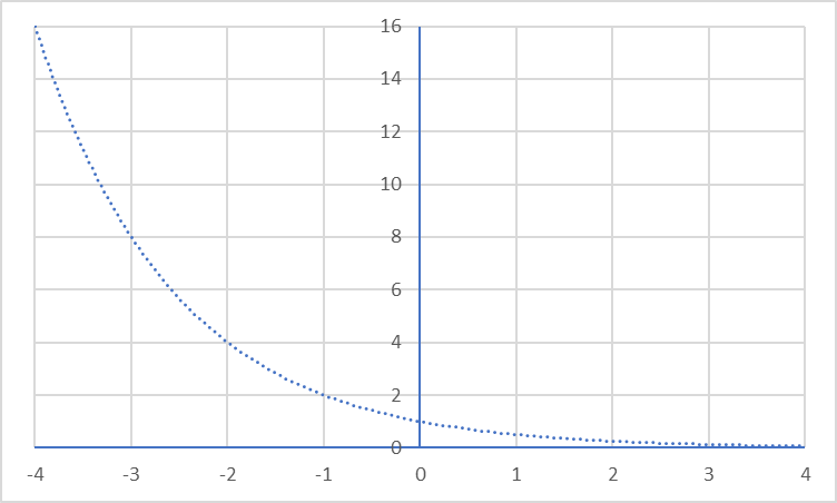
The same behaviour is exhibited by functions where the base of the function is a positive number less than 1.

Logarithmic plots

As mentioned earlier logarithmic plots can be useful to display data where there are large changes in magnitude. The pH scale is a good example of this. pH is a calculated as the negative base 10 logarithm of the molar hydrogen ion concentration of a solution:

pH = –log₁₀[H⁺]

However, logarithms also have another important function when displaying exponential data graphically. When you log transform a power function the result is a straight line. Consider the function:

$y = b^{x}$

If you take the log of both sides:

$\log_{10}y = \log_{10}b^{x}$

you can transform the equation to

$\log_{10}y = x\log_{10}b$

and then further simplify to

$y = xb$

which now has the form of straight line.

So, often a logarithmic scale for plotting exponential data as a straight line is easier to work with and a good test of whether the data is exhibiting exponential growth or decay.

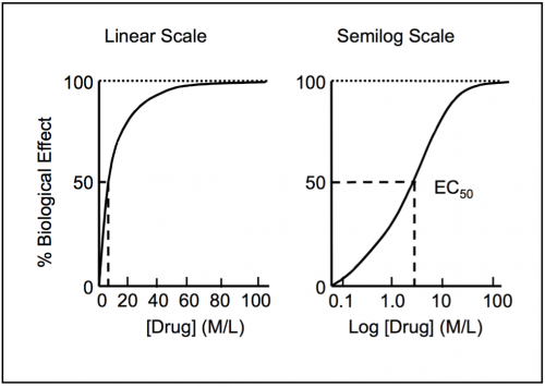
Example: Plotting data

The biological effects of drugs are not linear with dose and quite often more closely resemble an exponential function. Imagine increasing the dose of a drug that stimulates cardiac activity. For any drug there will be a lower limit (or threshold) which produces no biological effect (increased heart rate). Above this, the biological effect will start rapidly rising as the dose increases. However, there is a limited capacity for the heart to continually contract faster, so therefore there is an upper limit.

If we plot dose response curves on an arithmetic scale, they will be difficult to interpret as the points on the lower portion of the scale will be plotted close to one another. On a semi-logarithmic scale, as in the following chart, this is not the case, and it is much easier to determine parameters (such as EC₅₀ – the concentration of a drug that gives half-maximal response) that in turn are useful for comparing the effectiveness of similar drugs.

Two plots are shown using the same data for drug concentration vs biological effect. One is plotted using linear axes and the other uses a semi-log approach with a logarithmic axis for drug concentration. With a semi-log approach EC50 is much easier to discern. — Figure 12.5: Using a semi-log scale (right-hand plot) for a dose response curve makes it much easier to determine the EC50 – the concentration of a drug that gives half-maximal response compared to using a linear scale (left-hand plot). (From TUSOM | Pharmwiki used under CC BY-NC.)

License

Icon for the Creative Commons Attribution-NonCommercial-ShareAlike 4.0 International License

Foundations of Biomedical Science: Quantitative Literacy: Theory and Problems Copyright © 2023 by La Trobe University is licensed under a Creative Commons Attribution-NonCommercial-ShareAlike 4.0 International License, except where otherwise noted.

Euler’s number

e and the natural logarithm

What are logarithms?

Working with exponents

Multiplying like bases

Dividing like bases

Negative powers

Zero powers

Working with logs

Putting exponents and logs to use

Exponential decay

Logarithmic plots

Example: Plotting data

License

Share This Book