Appendix: Answers to problems

Julian Pakay

Appendix: Answers to problems

Chapter 2: Uncertainty in measurement and significant figures

1. 95.0°C – 3 significant figures
2. 120°C – 2 significant figures
3. 501 g – 3 significant figures
4. 15 patients – An exact number, so infinite
5. 0.450 ml – 3 significant figures
6. 250 mM – 3 significant figures
7. 2.38 × 10^-3 g – 3 significant figures
8. 0.00238 g – 3 significant figures
9. 2,050 mmol – 3 significant figures
10. 2.050 mmol – 4 significant figures
1. 1.22 M × 1.3 l = 1.586 mol – 1.6 mol
2. 500.00 g ÷ 125 ml = 4 g ml^–1 – 4.00 g ml^–1
3. 516.15 g − 0.005 g = 516.145 g – 516.14 g
4. 1.023 moles / 2.1 l = 0.4871 M – 0.49 M
5. 9.000 s − 0.5 s = 8.50 s – 8.5 s
6. The average height of 3 students with heights 170.3 cm, 167.23 cm and 171 cm
  (170.3 + 167.23 + 171) / 3 = 169.51 cm 170 cm

BOFFIN QUESTIONS: pH readings

pH = –log[H⁺]

pH = –log[2.56 × 10^–5]

pH = –(log[2.56] + log[10^–5]) (note that 2.56 has 3 significant figures)

pH = –(0.408 + –5) = 4.592

Following the rules for addition of significant figures:

0.408 has 3 significant figures, reflecting the uncertainty in the last digit of 2.56

while log 10^–5 = –5.0000 … has an infinite number of significant figures as 10^–5 is an exact number.

The rules of addition of significant figures state the number of places after a decimal point is less than or equal to the number of decimal places in every term in the sum.

So, the final answer is a pH of 4.592

Chapter 3: Estimation (sanity checking)

1. 37.7°C (to the nearest degree) – 38°C
2. 121 mM (to the nearest 10 mM) – 120 mM
3. 505.3 g (to the nearest 100 g) – 500 g
4. 505.3 g (to the nearest 10 g) – 510 g
5. 14.5 g l^–1 (to the nearest g l^–1) – 14.0 g l^–1
6. 0.0245 g (to the nearest mg) – 24 mg
7. 1.456 µg (to the nearest 100 ng) – 1,500 ng
1. 920 × 27 – (900 × 30 = 27,000)
2. 8,453 ÷ 53 – (8,450 ÷ 50 = 169)
3. 79 × 91 – (80 × 90 = 7,200)
4. 1,205 × 0.76 – (1,200 × 0.75 = 900)
5. 4,215 – 2,498 – (4,200 – 2,500 = 1,700)

BOFFIN QUESTIONS: Estimating large numbers

First, we need to work out the amount of protein in a HeLa cell.

We know the protein mass per volume is approximately 0.3 g/ml

We also know the volume of a HeLa cell is approximately 2,000 µm³

We need to convert µm³ into ml:

1 ml is 1 cm³

and 1 µm is 1 × 10^–4 cm

therefore 1 µm³ is 1 × 10^–4 cm × 1 × 10^–4 cm × 1 × 10^–4 cm = 1 × 10^–12 cm³

So, 2,000 µm³ = 2 × 10^–9 ml

So now we can determine the amount of protein in one cell:

0.3 g/ml × 2 × 10^–9 ml = 6 × 10^–10 g

We can work out the average molecular weight of HeLa cell proteins by multiplying the typical mass of an amino acid (110 Da) by the average length of HeLa proteins (400 amino acids) to give 44,000 Da (or g/mol).

Next we can calculate the number of moles of proteins per cell by dividing the mass of protein by the average molecular weight:

6 × 10^–10 g / 44,000 g/mol = 1.4 × 10^–14 mol

Finally, we can multiply this by Avogadro’s number (the number of molecules per mole) to determine the number of proteins:

1.4 × 10^–14 mol × 6 × 10²³ molecules/mol = 8 × 10⁹ protein molecules

Chapter 4: Biological scale

The mRNA molecule is certainly much larger! Proteins are made up of chains of amino acids. The average molecular weight of an amino acid is 110 Da while the average molecular weight of a ribonucleotide monophosphate (the monomer unit in an RNA molecule) is 327 Da. However, each amino acid in a protein is coded for by a triplet of nucleotides (each triplet is known as a codon). So, each nucleotide is 3 times bigger than an amino acid and there are at least 3 times more of them than amino acids in the corresponding protein, which is close to an order of magnitude (10-fold) difference in molecular weight.

If we think in spatial terms the difference in size between proteins and mRNA can be even greater. Proteins typically take on a more compact folded structure while RNA molecules tend to be more diffuse and linear, punctuated with secondary structures in the form of hairpins, stem-loops and pseudoknots.

The atomic radius is approximately 0.1 nm while the atomic nucleus is around 1 fm.

0.1 nm is 0.1 × 10^–9 m (1 × 10^–10 m) and 1 fm is 1 × 10^–15 m

This means that there is a difference of 1 × 10^–10 / 1 × 10^–15 = 100,000 or five orders of magnitude between them!

The scientific consensus is that this is not a coincidence! The endosymbiotic theory proposes that eukaryotic cells are the result of separate prokaryotic cells which joined together in a symbiotic union. At some point a free-living bacterium was engulfed by another cell and became the mitochondrion. The engulfed bacterium benefited from being in a protected nutrient-rich environment while the host cell benefited from the production of chemical energy by the symbiont. This endosymbiotic event occurred very early in the eukaryotic lineage as all eukaryotes contain mitochondria.

The evidence that supports this does not solely rely on size! Like bacteria, mitochondria have their own circular DNA, their own membranes, reproduce by fission, and some remnant protein components which are highly similar to those in bacteria.

The length of DNA in a human cell is therefore 6 Gbp × 0.3 nm bp^–1

That is, 6 × 10⁹ × 0.3 × 10^–9 m = 1.8 m!

This 1.8 m length of DNA must fit inside the cell’s nucleus, a space typically 5 µm across. This implies there must be a very efficient way of packing the DNA. The DNA is indeed packed into a series of higher order structures to form chromosomes. DNA initially bonds with proteins called histones to form chromatin. The DNA winds 1.65 times around a core nucleosome structure of 8 histone molecules. Theses nucleosomes fold to form a 30 nm wide fibre. This fibre then forms loops an average of 300 nm long. The loops are then compressed and folded to form a 250 nm wide fibre. This fibre is then coiled again to form the chromatids of the chromosome. The packing ratio from naked DNA to chromosomes is in the order of 10,000:1!

BOFFIN QUESTIONS: Fantastic Voyage

Based on the width of a human arm, we might generously estimate that Raquel’s eyes (pupils) are about 1/10th the width of the hair cell cilia. That would make them 0.02 µm in diameter, which is 20 nm. The human eye can detect wavelengths of light from 380 to 700 nm. This means that Raquel’s eyes, being much smaller than the wavelength of visible light, will not allow her to see at all!

This is not the only scientific fault with this film. However, if you can suspend disbelief and get past some of the outdated special effects it is still a lot of fun!

To solve this, you first need to convert both heights to same units:

3 µm = 3 × 10^–6 m

Therefore, the volume decrease will be (3 × 10^–6/1.8)³ = 4.6 × 10^–18

If their starting mass stays the same, then their density would be 2.16 × 10²⁰ kg m^–3

This is far denser than the Earth’s core! If there was a way to shrink people like this they would sink through the floor, bedrock and all the way through the Earth’s mantle!

Chapter 5 Scientific notation and SI units

1. 123,000 m – 1.23 × 10⁵ m
2. 299 l – 2.99 × 10² l
3. 0.0035 mol – 3.5 × 10^–3 mol
1. 0.004 mol to mmol – 4 mmol
2. 1.76 ml to µl – 1,760 µl
3. 0.0023 µm to nm – 2.3 nm
4. 20.3 µl to l – 2.03 × 10^–5 l
5. 0.12 fg to ng – 1.2 × 10^–7 ng
6. 1.2 nmol to pmol – 1,200 pmol
7. 1.2 mg µl^–1 to g l^–1 – 1.2 mg µl^–1 = 0.0012 g µl^–1 = 1,200 g l^–1
8. 1.2 ng µl^–1 to g l^–1 – 0.0012 g l^–1

BOFFIN QUESTIONS: How many cells are in your body?

To solve this, you need the volume of your body to be in the same units as the volume of a cell. In this case the volume of the body will be converted into µm³.

Assuming the mass of the body is 70 kg, 1 kg takes up about 1 l so the volume is 70 l.

1 L is 0.001 m³ so the total volume is 0.07 m³

1 m = 1 × 10⁶ µm

Therefore, 1 m³ = 1 × 10¹⁸ µm³

The volume of the body is 0.07 × 1 × 10¹⁸ µm³ = 7 × 10¹⁶ µm³

Now the number of cells can be calculated:

7 × 10¹⁶ µm³ / 1 × 10³ µm³ cell^–1 = 7 × 10¹³ cells

7 × 10¹⁶ µm³ / 1 × 10⁴ µm³ cell^–1 = 7 × 10¹² cells

The answer is there are between 7 × 10¹² and 7 × 10¹³ cells in a 70 kg body. So the answer is between 7 trillion and 70 trillion cells.

It is worth reading the paper by Sender et al. (2016) to see how they approach calculating an estimate regarding the total weight of bacteria in the human body.

They use a 70 kg ‘reference man’ to make their estimate. They obtain estimates of the total number of bacteria from human tissues and conclude that compared to the colon the total number of bacteria is negligible. So, the focus of their calculation is the volume of the colon and the concentration of bacteria within.

They estimate that the volume of the colon is 0.4 l (corresponding to 400 g) and the number of bacteria per gram of wet stool is 0.9 × 10¹¹. This gives them an estimate of 3.6 × 10¹³ bacteria in the colon and considering that the contribution to the total number of bacteria from other organs is at around 10¹², they use 3.8 × 10¹³ as their estimate for the number of bacteria across the whole body for their reference man.

Since bacteria make up about 50% of the mass of the content of the colon, an estimate of their total weight is 200 g. This number is consistent with the accepted estimate of the wet weight of a bacterium being 5 pg.

Total weight of bacteria = 3.8 × 10¹³ bacteria × 5 pg per bacterium

Total weight of bacteria = 3.8 × 10¹³ bacteria × 5 × 10^–12 g per bacterium

Total weight of bacteria = 190 g (approximately 200 g)

This total mass of bacteria mass represents about 0.3% of the overall body weight.

Percentage by weight of bacteria in a human is (0.2 kg / 70 kg) × 100 = 0.3%

Chapter 6: Composition of blood

In order to estimate the platelet concentration of the suspension you need to determine the number of platelets present in a defined region of the haemocytometer, then calculate the volume that region encompasses.

Cells in the central 16 squares are counted. But what to do with cells overlapping the outside borders of those 16 squares? The best way to accurately count is to use a consistent approach such as counting only those cells on the border for the top and right borders and excluding those on the bottom and left borders. Normally for an accurate determination of cell numbers, multiple counts are made, and an average is taken.

The cell count obtained is 102 platelets. (If your estimate is slightly different do not be too concerned – there will be an operator error with this kind of estimate.)

The volume of the 16 central squares is 0.2 mm × 0.2 mm × 0.1 mm = 0.004 mm³

We need to now convert that volume to ml. Often it is easier to start with the base units and work towards your values:

1 m³ = 1,000 l

0.001 m³ = 1 l

1 × 10^–6 m³ = 1 ml

Remember that units of volume are the cubes of units of length:

1 m³ = 1 × 10⁹ mm³

So, from above, 1 ml = 1 × 10^–6 × 1 × 10⁹ mm³ = 1,000 mm³

Therefore, the volume in ml of the 16 central squares of the haemocytometer is:

0.004/1,000 = 4 × 10^–6 ml

So now we can calculate the platelet concentration:

102 platelets / 4 × 10^–6 ml = 2.55 × 10⁷ platelets/ml

The leukocyte in the micrograph is roughly 1.5 times the diameter of the erythrocytes. Given that erythrocytes are typically around 6–8 µm, this would make the cell around 9–12 µm in diameter. This size and the secretory granules contained within the cell are consistent with a type of granulocyte known as a mast cell.

Chapter 7: Solutions and concentrations

Molarity (M) refers to concentration in moles per litre. In this case you can use the equation:

C = n/V

where

C = molar concentration (M)

n = number of moles

V = volume (l).

Therefore, C = 5 mol / 2.5 l = 0.2 M

This is a two-step problem. First you need to determine the number of moles using the mass of NaOH and the molecular weight:

Number of moles = mass/molecular weight = 5 g/40 g mol^–1 = 0.125 mol

Then you can use the number of moles and the volume to determine the molarity. The volume needs to be converted from ml to L:

750 ml = 0.75 l

C = 0.125 mol/0.75 l = 0.17 M = 170 mM

C = n/V

Therefore, M = n / 10 l

n = 2 M × 10 l = 20 mol

This is a two-step problem. First you need to determine the moles of Na2CO3 using the molarity and the volume. Remember that the volume should be converted to l and the concentration should be converted to M.

C = 100 mM = 0.1 M

V = 750 ml = 0.75 l

C = n/V

M = n / 0.75 L

n = 0.075 mol

Then you can use the number of moles and the molecular weight to work out the mass required:

Mass = number of moles × molecular weight = 0.075 mol × 106 g mol^–1 = 7.95 g

In this problem we first need to work out the mass of cholesterol in 1 l.

There is 0.1 l in 1 dl

Therefore, the cholesterol concentration (mg l^–1) is 10 × 97 mg = 970 mg l^–1

Next, we can use the mass and the molecular weight to determine the number of moles per litre (molarity). Remember that the mass must first be converted to g.

Moles = 0.970 g / 386.64 g mol^–1 = 0.0025 mol

Therefore, the molarity is 0.0025 M = 2.5 mM

Moles of HCl in 90 ml of a 3 M solution = 0.09 l × 3.0 M = 0.27 mol

Mass = number of moles × molecular weight = 0.27 mol × 36.46 g mol^–1 = 9.8 g

First you need to convert mg to g:

50 mg = 0.05 g

Then, use the mass and molecular weight to determine the number of moles:

Number of moles = mass / molecular weight = 0.05 g / 100.1 g mol^–1 = 5 × 10^–4 mol = 0.5 mmol

First you need to determine the mass present in 1 l:

5 µM = 5 × 10^–6 M = 5 × 10^–6 mol l^–1

Mass per litre = moles per litre × molecular weight

Mass per litre = 5 × 10^–6 mol l^–1 × 27,000 g mol^–1 = 0.135 g l^–1

1 g l^–1 = 1 mg ml^–1

So the final answer is 0.135 mg ml^–1

First you need to determine the number of moles present in 1 ml. You need to convert the volume to l and the molarity to M:

1 ml = 0.001 l

50 nM = 5 × 10^–8 M

n = CV = 0.001 L × 5 × 10^–8 M = 5 × 10^–11 mol

Once you have determined the number of moles you can use this and the molecular weight to determine the mass:

The molecular weight is 60 kDa, which = 60,000 Da, which = 60,000 g mol^–1

Mass = number of moles × molecular weight = 5 × 10^–11 mol × 60,000 g mol^–1 = 3 × 10^–6 g

3 × 10^–6 g = 3 × 10^–3 mg = 3 µg

Assume 1 ml is the equivalent of 1 g

Therefore, the mass required is 300 × 60/100 = 180 g

There are 45 g in 2 l

Assume 1 ml is the equivalent of 1 g, so convert the volume from l to ml

Therefore, the weight/volume percentage concentration is:

45/2,000 × 100 = 2.25%

For this question assume that the volumes are completely additive.

Volume of benzene = 30 ml

Total volume = 30 ml + 95 ml = 125 ml

The percent volume of benzene = 30/125 × 100 = 24%

Mass = concentration × volume

Amount of ampicillin = 50 µg ml^–1 × 150 ml = 7,500 µg = 7.5 mg

$\text{Parts per million (ppm)} = \frac{ \text{mass solute}}{\text{mass of solution}} \times 10^{6}$

Assume 1 ml = 1 g

So, 0.1 l = 100 ml = 100 g

ppm = 0.025 g / 100 g × 10⁶ = 250

$\text{ppb} = \frac{\text{mass solute}}{\text{mass of solution}} \times 10^{9}$

Substituting into the equation above:

$130 = \frac{\text{mass of dissolved nitrates}}{600g} \times 10^{9}$

Mass of dissolved nitrates = (600 × 130)/10⁹ = 7.8 × 10^–5 g = 0.078 mg = 78 µg

$\text{ppm} = \frac{\text{mass solute}}{\text{mass of solution}} \times 10^{6}$

Convert the volume to mass:

1 l = 1,000 ml = 1,000 g

Substituting this into the equation above:

$5 = \frac{\text{mass solute}}{1,000} \times 10^{6}$

Mass of solute = (5 × 1,000)/10⁶ = 0.005 g = 5 mg

BOFFIN QUESTIONS: Determining an unknown concentration

To determine the concentration of the ATP solution, substitute the values into the Beer’s law equation (A = εbc) and solve for c:

0.8 = 15,400 M^–1 cm^–1 × 1 cm × c

c = 0.8 / 15,400 M^–1 cm^–1 × 1 cm

c = 5.2 × 10^–5 M = 0.052 mM = 5.2 µM

To calculate the unknown cholesterol concentration, you can use the standard curve’s equation, substituting the absorbance for y and solving for x (µg ml^–1 cholesterol):

$y = 0.003x - 0.1648$

$0.865 = 0.003x - 0.1648$

$x = (0.865 + 0.1648) / 0.003 = 343 \text{µg ml}^{-1} \text{cholesterol}$

Chapter 8: Dilutions

To solve this, use the equation:

C₁V₁ = C₂V₂

In this case you need to determine the volume of the initial solution required (V₁):

2 M × V₁ = 0.3 M × 400 ml

V₁ = (0.3 M × 400 ml) / 2 M = 60 ml

To solve this, use the equation:

C₁V₁ = C₂V₂

However, you first need to convert the concentrations to the same units:

800 mM = 0.8 M

2 M × V₁ = 100 μl × 0.8 M

V₁ = (100 μl × 0.8 M) / 2 M = 40 μl

Use the equation C₁V₁ = C₂V₂ solving for C₂

You need to also calculate the final volume (V₂) in this case as 50 µl + 825 µl = 875 µl

0.5 M × 50 µl = C₂ × 875 µl

C₂ = 0.029 M = 30 mM

Use the equation C₁V₁ = C₂V₂ solving for V₁

11.6 M × V₁ = 100 ml × 0.1

V₁ = 0.86 ml = 860 µl

Use the equation C₁V₁ = C₂V₂ solving for V₂

250 ml × 1.25 = 0.25 × V₂

V₂ = 1,250 ml

Use the equation C₁V₁ = C₂V₂ solving for C₂

450 ml × 0.2 M = C₂ × 225 ml

C₂ = 0.4 M

The dilution factor is the total volume (V2) / initial volume (V1). Note that since this is a ratio it is important that both volumes are in the same units.

Dilution factor = (38.75 ml + 0.25 ml) / 0.25 ml = 156 (or a 156-fold dilution)

Use the equation C₁V₁ = C₂V₂ solving for V₁

The fact that there is 2 L of 0.25 M Na₂CO₃ is not relevant to the problem unless it is an insufficient amount to prepare the final solution!

0.25 M × V₁ = 100 ml × 0.1 M

V₁ = 40 ml

This is a serial dilution as two consecutive dilutions have been made. To determine the final concentration the two separate dilution factors can be determined and multiplied to provide the overall dilution. Then the initial concentration can be divided by this factor to determine the final concentration. Remember to convert volumes to the same units when calculating the dilution factors.

1st dilution factor = (50 µl + 350 µl) / 50 µl = 8

2nd dilution factor = (25 µl + 1,250 µl) / 25 µl = 51

Total dilution factor = 8 × 51 = 408

Final BSA concentration = 10 mg ml^–1/408 = 0.025 mg ml^–1 = 25 µg ml^–1

Use the equation C₁V₁ = C₂V₂ solving for V₁

Note that the concentration 10x is a suggested dilution so you can assume the final concentration should be 1x.

$10x \times V_{1} = 1x \times 50 \text{µl}$

$V_{1} = 5 \text{µl}$

In this case, the stated concentration is not relevant to the problem – only the dilution factor matters.

Dilution factor = V₂ ÷ V₁

10 = (1 ml + x) / 1 ml

x = 9 ml

That is, 9 ml of water needs to be added to 1 ml to achieve a 10-fold dilution.

There are two serial dilutions made here. To find the overall dilution factor, which requires working back to the original concentration of the analyte, you need to multiply the two individual dilution factors.

Dilution factor = (100 µl + 300 µl) / 100 µl = 4

Since this was done twice the overall dilution factor is 4 × 4 = 16

The first part of the question can be reworded:

Since there is 0.75 mg of DNA in 1 ml, what volume will contain 50 pg?

Since you are working with ratios the units must be the same. So, you can convert pg to mg or mg to pg:

0.75 mg = 750 µg = 750,000 ng = 750,000,000 pg = 7.5 × 10⁸ pg

Volume containing 50 pg = (50 pg / 7.5 × 10⁸ pg) × 1 ml = 6.67 × 10^–8 ml

6.67 × 10^–8 ml = 6.67 × 10^–5 µl

This is far too small a volume to pipette! The DNA solution first needs to be diluted.

To determine the dilution factor required divide the original concentration by the final concentration.

From above, the original concentration was 7.5 × 10⁸ pg ml^–1 = 7.5 × 10⁵ pg µl^–1

The final concentration required is 50 pg in 2.5 µl (i.e. 10% of 25 µl) = 20 pg µl^–1

The dilution factor required is 7.5 × 10⁵ pg µl^–1/20 pg µl^–1 = 37,500

You could achieve this dilution by adding 1 µl of the original DNA to 37.5 ml of water or preferably do this by a serial dilution. There are infinite ways to solve this. Here is one possible solution which minimises volumes:

1. Dilute the original solution by adding 100 µl to 900 µl of water (dilution = 10)
2. Dilute the previous solution 10-fold by adding 100 µl to 900 µl of water
  (overall dilution = 100)
3. Dilute the previous solution 10-fold by adding 100 µl to 900 µl of water
  (overall dilution = 1,000)
4. Dilute the previous solution 10-fold by adding 100 µl to 900 µl of water
  (overall dilution = 10,000)
5. Dilute the previous solution 3.75-fold by adding 100 µl to 275 µl of water
  (overall dilution = 37,500)

BOFFIN QUESTIONS: Homeopathy

Without randomised control trials it is very difficult to test the effectiveness of homeopathy as this is the best way to isolate the variable of receiving the homeopathic treatment. The current scientific consensus is that when randomised control trials have been conducted, they have shown that the effectiveness of homeopathic treatment is indistinguishable from the placebo^[1].
First, you need to determine the concentration of aescin in the original preparation.

Since aescin is 30% by weight of the seeds, 10 mg ml^–1 of ground Aesculus hippocastanum seeds should contain 3 mg ml^–1 aescin.

From this and the molecular weight of aescin you can determine its molar concentration:

3 mg ml^–1 = 3 g l^–1

Number of moles = mass / molecular weight

Number of moles = 3 g / 1131.26 g mol^–1 = 2.652 × 10^–3 mol

Therefore, the preparation is 2.652 × 10^–3 M

This preparation is diluted 18 times, which is actually 1 × 10¹⁸

Therefore, the concentration of the homeopathic treatment is:

2.652 × 10^–3 M / 1 × 10¹⁸ = 2.652 × 10^–21 M

To determine the number of molecules of aescin in a 1 ml aliquot, determine the number of moles found in 1 ml and then multiply by Avogadro’s number (6.022 × 1023):

2.652 × 10^–21 M = 2.652 × 10^–21 mol L^–1 = 2.652 × 10^–24 mol ml^–1

Number of molecules per ml = 2.652 × 10^–24 mol × 6.022 × 10²³ = 1.6

At this concentration the homeopathic preparation approaches a Poisson distribution as to whether it contains a single molecule of aescin!

Side Bar – A Poisson distribution is a discrete probability distribution. It gives the probability of an event happening a certain number of times within a given interval of time or space and often used to describe the distribution of rare events in a large population.

Chapter 9: Medical diagnostics – Measurement, uncertainty and distributions

1. Mean = 20.1
2. Mode = 17
3. Range = 8 (25–17)
To compare you need to determine the coefficient of variation for each standard. Use the formula:

$cv = \frac {s}{\overbar{x}}\times 100$

cv_(high) = 0.051/1.005 × 100 = 5.07%

cv_(low) = 0.006/0.104 × 100 = 5.77%

The assay is more precise at the higher standard concentration.

Since this is a reference interval for the general population a major consideration is to have a large enough sample to provide a reasonable estimate of the distribution of the analyte. Also, the subjects being tested (the reference population) should be as similar as possible to the population (in this case the general population) for which the test will be applied, except for the presence of disease. The major factors normally considered are age and sex but there could be racial or environment factors such as socio-economic status that could be taken in consideration along with common health factors such as obesity or diabetes.

BOFFIN QUESTIONS: Do ACE inhibitors increase susceptibility to COVID-19?

The key to understanding why this data might be flawed is the self-reporting aspect. People who have hypertension and are prescribed ACE inhibitors are likely to monitor their health more fastidiously than the general population. They are less likely to ignore symptoms and, being in an already high-risk group, more likely to get tested for COVID-19 infection. This highlights a common flaw in observational or self-reporting studies.

Despite the flaws in these early studies, this correlation did lead some clinicians to initially advise patients to stop taking prescribed ACE inhibitors. However, more rigorous clinical studies demonstrated that there was no evidence of ACE inhibitors increasing the chances of developing COVID-19 or affecting its severity. In fact, patients are more at risk of developing complications from COVID-19 without these medications due to increased hypertension.

Chapter 10: Medical diagnostics – Sensitivity and specificity

	Target disorder (strep tonsillitis)
		Present	Absent	Totals
Diagnostic test result	Positive RST	159	3	162
	Negative RST	36	1,302	1,338
Total		195	1,305	1,500

Sensitivity = true positives / (true positives + false negatives) × 100

Sensitivity = 159 / (159 + 36) × 100 =81.5%

Specificity = true negatives / (true negatives + false positives) × 100

Specificity = 1,302 / (1,302 + 3) × 100 = 99.8%

1. Sensitivity = true positives / (true positives + false negatives) × 100
  92 = x/500 × 100
  x = 460
  That is, 460 of the positives would test positive.
2. Specificity = true negatives / (true negatives + false positives) × 100
  94 = x/500 × 100
  x = 470
  That is, 470 of the negatives would test negative.

	Disease
		Present	Absent	Totals
Diagnostic test result	Positive	192	7,984	8,176
	Negative	8	91,816	91,824
Total		200	99,800	100,000

Sensitivity = true positives / (true positives + false negatives) × 100

96 = x/200 × 100

True positives = 192

Specificity = true negatives / (true negatives + false positives) × 100

92 = x/99,800 × 100

True negatives = 91, 816

1. 1. 192/8,176 × 100 = 2.35%
  2. 91,816/99,800 × 100 = 92% (note the definition of specificity)

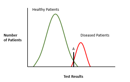
Since COVID-19 is a serious illness with the added problem of being highly contagious, it would be better to shift the threshold to the left. That is, increase sensitivity but reduce specificity. It would result in an increase in false positives but ensure that all diseased individuals can be quarantined. Follow-up diagnostic tests would be required to clear the false positives.

Chapter 11: Correlation, causation and confounding variables

The answer is (b) r = –0.5.
No, this is not correct. Blood type is categorical data and cannot be used to determine correlation. Both variables need to be continuous or on an interval scale. One variable should also be normally distributed, and the data should follow a linear relationship.
No, to determine how much the degree of late gadolinium enhancement explains the variation in troponin I levels you need to use the coefficient of determination, R². In this case it is (0.52)2 = 0.27. So, it would be correct to say that based on the data, the degree of late gadolinium enhancement explains 27% of the variation in troponin I levels. It is important to remember not to confuse the correlation coefficient (r or R) with the coefficient of determination (r² or R²).
While latitude will directly correspond to the amount of sunlight and it is plausible to suggest that the amount of sunlight might explain the incidence of skin cancer there could be many cofounding variables which account for this correlation. For example, there could be demographic differences in the people living at the different latitudes. Different ethnicities of populations at different latitudes may have different genetic profiles which either protect them from or render them more susceptible to skin cancer. Likewise, there could be differences in diet at different latitudes. These could be potentially controlled for by careful analysis of the data.
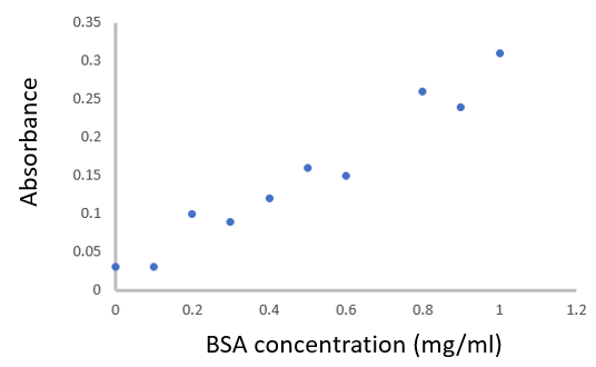
1. For the plot, BSA concentration is the independent variable (set by the experimenter) and by convention is plotted on the x-axis, while absorbance is the dependent (measured) variable and by convention is plotted on the y-axis.

1. b. To determine the correlation coefficient (r), you could use Excel or another program to calculate this for you. Your answer should be close to 0.98 – a very strong positive correlation! Remember not to confuse the correlation coefficient (r) and the coefficient of determination (R²). You can also calculate the correlation coefficient manually.

x	y	x – xmean	y – ymean	(x – x_mean)²	(y – y_mean)²	Cross product
0	0.03	–0.48	–0.119	0.2304	0.014161	0.05712
0.1	0.03	–0.38	–0.119	0.1444	0.014161	0.04522
0.2	0.1	–0.28	–0.049	0.0784	0.002401	0.01372
0.3	0.09	–0.18	–0.059	0.0324	0.003481	0.01062
0.4	0.12	–0.08	–0.029	0.0064	0.000841	0.00232
0.5	0.16	0.02	0.011	0.0004	0.000121	0.00022
0.6	0.15	0.12	0.001	0.0144	0.000001	0.00012
0.8	0.26	0.32	0.111	0.1024	0.012321	0.03552
0.9	0.24	0.42	0.091	0.1764	0.008281	0.03822
1	0.31	0.52	0.161	0.2704	0.025921	0.08372
x̅ = 0.48	x̅ = 0.149	∑ = 0	∑ = 0	∑ = 1.056	∑ = 0.08169	∑ = 0.2868

We can now put these values into the correlation coefficient equation:

$\displaystyle r = \frac{n(\sum xy) - (\sum x)(\sum y)}{\sqrt{n \sum x^{2} - (\sum x)^{2}} \sqrt{n \sum y^{2} - (\sum y)^{2}}}$

$\displaystyle r = \frac{0.2868}{(\sqrt{1.056})(\sqrt{0.08169})}$

$\displaystyle r = 0.976$

c. You can use Excel or another program to calculate this for you. When using Excel, you can fit a trendline to the data. You should choose a linear trendline and the equation of the line should be close to:

y = 0.2716x + 0.0186

That is, absorbance = 0.2716 (BSA concentration in mg/ml) + 0.0186

When fitting a trendline you will be given the option of forcing the line through the origin (0,0). While 0,0 is a valid data point you should not force the line through this point. Rather, you want a line of best fit.

d. Now that you have an equation for the trendline or line of best fit you can use this to calculate the concentrations of unknown solutions. For a solution with an absorbance of 0.135 the expected concentration would be:

Absorbance = 0.2716 (BSA concentration in mg/ml) + 0.0186

0.135 = 0.2716 (BSA concentration in mg/ml) + 0.0186

0.135 – 0.0186 = 0.2716 (BSA concentration in mg/ml)

0.1164/0.2716 = BSA concentration in mg/ml

BSA concentration = 0.43 mg/ml

e. The additional data points illustrate an important consideration for standard curves, which is that it is not valid to extrapolate beyond the range of the standards used to create the standard curve. For example, there may be a strong linear correlation between the dependent and independent variable, but this will not necessarily hold true when the value of the independent variable increases. In this case the additional data points with higher BSA concentrations do not appear to fit the trendline. Absorbance plateaus around 0.36–0.37 at BSA concentrations of 1.4 mg/ml or above.

Practically this means that if you used the original trendline to estimate the BSA concentration of a solution with an absorbance of 0.37 there would be a danger of greatly underestimating the actual BSA concentration.

BOFFIN QUESTIONS: Football and COVID-19 – A correlation?

It is unlikely that being good at football leads to an increased risk of catching or spreading COVID-19. It is also not plausible that COVID-19 makes you a better footballer and, besides, the FIFA ranking data predates the emergence of COVID-19. However, this does not mean that the data is necessarily spurious and correlations, while not always directly linked to causation, are worth investigating.

So how could these variables be linked? There are many possibilities:

- Where football is popular there are more mass gatherings due to football matches, which contributes to the spread of COVID-19.
- A nation’s football ranking may be linked to economic status and a better football ranking correlates with increased travel or increased social activity, which leads to increased spreading.
- Conversely, many poorer nations may not be as good at football and as they are poorer they are less able to test for COVID-19, so the infection rate is under-reported.

To establish a causal link, all of these variables would need to be investigated.

Chapter 12: Growth and decay – Exponents and logarithms

To solve this, you can use the general rule for dividing exponents:

$y^{m} ÷ y^{n} = y^{m-n}$

Therefore, the answer is $x^{9-3} = x^{6}$

To convert between logarithmic and exponential forms you can use the general rule:

$log_{b}(M) = N M = b^{N}$

In this case, $x = 3^{9} \text{is converted to} \log_{3} x = 9$

$\log_{10} 1,000 = 3$
$x^{z} = y$
$3^{0} = 1$
This is an important rule – any number raised to the power of 0 is equal to 1.
You can solve this using the general rule:

$\log_{y}(y^{x}) = x$

or by performing the conversion below (a useful operation when solving for unknown exponents).

$\log_{c} x^{n} = n \log_{c} x$

$\log_{5} 5^{p} = p \log_{5} 5 = p<span style="font-size: 14pt">$

True
False; in this case the answer is $\log a / \log b<span style="font-size: 14pt">$
True, following the general rule:
$\log_{c} x^{n} = n \log_{c} x$
False; think about how $\log_{10}10^{2}$ differs from $(\log_{10}10)^{2}$

$\log_{10}10^{2} = 2 \log_{10} 10 = 2$

but

$(\log_{10} 10)^{2} = (\log_{10}10) \times (\log_{10}10) = 1$

To solve for x, use the general rule to get the equation into an exponential form:

$\log_{b} (M) = N \text{can be converted to} M = b^{N}$

$\ln x = -3$

can be written as:

$\log_{e} x = -3$

x = 0.0498

To solve for an unknown exponent, take the log of both sides to isolate the exponent:

$7 x = 287$

$\ln 7^{x} = \ln 287$

$x \ln 7 = \ln 287$

$x = \ln 287 / \ln 7$

$x = 5.66/1.96 = 2.91$

You can just go ahead and plug this into a calculator or first simplify using the general rule:

$\log_{2} \frac{x}{y} = log_{2}x - \log_{2}y$

So

$\ln \frac{1}{\sqrt{e}} = \ln 1 - \ln \sqrt{e} = 0 - 0.5 = -0.5$

There is a logarithmic relationship between hydrogen ion concentration and pH where:

$\text{pH} = - \log_{10}[ \,\text{H}^{+}] \,$

$[ \,\text{H}^{+}] \,$

is the hydrogen ion concentration in mol L^–1

To solve for [H⁺] given the pH, convert the logarithmic equation into an exponential equation:

$[ \,\text{H}^{+}] \, = 10^{- \text{pH}}$

Therefore, at pH 7.4, [H⁺] is:

$10^{-7.4} = 3.98 \times 10^{-8} \text{mol} L^{-1}$

The answer is (a), in which 50 represents the starting number of bacteria. This is multiplied by 2 since they are doubling with each time increment. t is equal to time in hours and this needs to be multiplied by 3 since they double every 20 minutes (3 times per hour). The other equations are incorrect as they either do not include the starting population or fail to incorporate the doubling at each time increment.
You can use this information to write an equation for the number of bacteria at time d (days of 24 hours):

$\text {Number of bacteria (at time} d) = 1,000(2)^{3d}$

Since the population doubles every 8 hours then this will occur 3 times per day.

$\text{Number of bacteria (at time} d) = 1,000(2)^{3(2.5)} ~ 180,000$

a.

$Z(t) = \frac {50,000}{(2 + e^{10-5})}$

$Z(5) = \frac{50,000}{(2 + e^{5})}$

$Z(5) = \frac{50,000}{(2 + 148.41)}$

$\text{Zombies at 5 days} = 332$

b.

As t approaches infinity, $e^{10-t}$ approaches 0, so the equation becomes 50,000/2 = 25,000

So, 25,000 is the maximum number of people that can turn into zombies.

By substituting 900 into the equation for RR, the answer is 396 ms.
Substitute 330 for QT:

$330 = 425 - 676e^{-0.0037.RR}$

$676e^{-0.0037.RR} = 95$

$e^{-0.0037.RR} = 95/676$

To solve for RR take the natural logarithm of both side of the question:

$\ln⁡(e^{-0.0037.RR}) = \ln⁡ \left( \frac{95}{676} \right)$

$\text{RR}=\frac{\ln{\frac{95}{676}}}{-0.0037}~ 503$

Therefore, a QT of 330 ms corresponds to RR of approximately 530 ms

$A = A_{0}e^{-0.05t}$

$2 = 4e^{-0.05t}$

$0.5 = e^{-0.05t}$

$\ln 0.5 = \ln ^{e-0.05t}$

$\ln 0.5 = -0.05t \ln e$

$\frac{-0.693}{-0.05 \ln e} = t$

$t = \frac{-0.693}{-0.05}$

$t = 13.9 \text{days}$

BOFFIN QUESTIONS: Exponential bias

Let’s use rice instead of wheat. One grain of rice is placed in the first square. This will double for each square. Since there are 64 squares in total there are 63 doublings.

Grains of rice = 1 × 2⁶³ = 9,223,372,036,854,775,808 grains!

The average weight of 1 grain of rice (from a sample of short, medium and long grains) is 21 mg. Therefore, the total weight of rice is:

0.021 g × 9,223,372,036,854,775,808 = 193,690,812,773,950,292 g = 193,690,812,774 tonnes

To put this in perspective current worldwide annual production is around 740,000,000 tonnes!

The answer here is subjective. Many people may not realise this is the same data but with either a linear y-axis (graph A) or an exponential y-axis (graph B). If only data for the initial period was available, then graph B might be more effective to convince the general population to practice social distancing as this graph clearly shows the increase over time while in graph A the number of infections appears static. However, when looking at the entire time course the exponential nature of the increase in infection over time in graph A is probably more obvious to a casual observer.
This question highlights the fact that a small change to a parameter in an exponential function can produce a very large effect.
1. First you need to develop an equation to model the growth in infections.

Number of people initially infected = 23

No handwashing growth rate expressed as a decimal = 0.28

Handwashing growth rate expressed as a decimal = 0.23

Final number of people infected = 1,000,000

Time (days) = t

No handwashing

$1,000,000 = 23(1+0.28)^{t}$

$43,478.3 = 1.28^{t}$

$\ln 43,478.3 = \ln 1.28^{t}$

$t = \frac{\ln 43,478.3}{\ln 1.28}$

$t = 43.3 \text{days}$

Handwashing

$1,000,000 = 23 (1+0.23)^{t}$

$43,478.3 = 1.23^{t}$

$\ln 43,478.3 = \ln 1.23^{t}$

$t = \frac{\ln 43,478.3}{\ln 1.23^{t}}$

$t = 51.5 \text{days}$

Handwashing buys 8.2 days!

b. The same formula can be used for this question but in this case we know the time period (30 days) and need to work out the number of infections.