11.3 Calculating the correlation coefficient (r)
The correlation coefficient (r) is defined as how close a set of data points associate with a line (linear regression line) based on those points. You calculate it by taking the ratio of the covariance of the two variables normalised to the square root of their variances. Practically, you are unlikely to calculate this value by hand, especially for a large dataset, but it can be of value to follow a calculation to understand how this coefficient is derived. The formula is:

So, to calculate r for the data for graph A in the previous figure, first calculate the mean.
| x | y | |
| 1 | 2 | |
| 3 | 4 | |
| 4 | 7 | |
| 5 | 5 | |
| 6 | 7 | |
| 7 | 9 | |
| 8 | 10 | |
| Mean | 4.86 | 6.29 |
Now you can calculate the deviation from the mean for each of the values followed by the square of each.
| x | y | x – xmean | y – ymean | (x – xmean)2 | (y – ymean)2 |
| 1 | 2 | –3.9 | –4.3 | 14.9 | 18.4 |
| 3 | 4 | –1.9 | –2.3 | 3.4 | 5.2 |
| 4 | 7 | –0.9 | 0.7 | 0.7 | 0.5 |
| 5 | 5 | 0.1 | –1.3 | 0.0 | 1.7 |
| 6 | 7 | 1.1 | 0.7 | 1.3 | 0.5 |
| 7 | 9 | 2.1 | 2.7 | 4.6 | 7.4 |
| 8 | 10 | 3.1 | 3.7 | 9.9 | 13.8 |
|
x̅ = 4.9
|
x̅ = 6.3
|
∑ = 0 | ∑ = 0 | ∑ = 34.9 | ∑ = 47.4 |
Now you calculate the sum of the cross product of these deviation scores (e.g. for the first line this is –3.9 × –4.3).
| x | y | x – xmean | y – ymean | (x – xmean)2 | (y – ymean)2 | Cross product |
| 1 | 2 | –3.9 | –4.3 | 14.9 | 18.4 | 16.5 |
| 3 | 4 | –1.9 | –2.3 | 3.4 | 5.2 | 4.2 |
| 4 | 7 | –0.9 | 0.7 | 0.7 | 0.5 | –0.6 |
| 5 | 5 | 0.1 | –1.3 | 0.0 | 1.7 | –0.2 |
| 6 | 7 | 1.1 | 0.7 | 1.3 | 0.5 | 0.8 |
| 7 | 9 | 2.1 | 2.7 | 4.6 | 7.4 | 5.8 |
| 8 | 10 | 3.1 | 3.7 | 9.9 | 13.8 | 11.7 |
|
x̅ = 4.9
|
x̅ = 6.3
|
∑ = 0 | ∑ = 0 | ∑ = 34.9 | ∑ = 47.4 | ∑ = 38.3 |
We can now put these values into the equation:


A very strong positive correlation!
Note
To calculate the correlation coefficient, the data for both variables should be continuous or on an interval scale (you cannot calculate the correlation coefficient for categorical data). Also, the data for at least one variable should be normally distributed and should have a linear relationship – which can be read from looking at a scatter plot of the data.
Calculating linear regression
We can also use these values to help calculate the line of regression (line of best fit for the data points).A straight line can be described using the equation:

where a = the intercept and b = the slope of the line.
The slope can be determined by the following equation:

Therefore, in this example:


We can then calculate the intercepts by substituting the mean values for x and y into our linear regression equation:


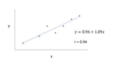
So now our equation is:

And we could represent the data using the following graph.