45 Where does the Normal Distribution Model come from?

Knowing where the model comes from will help us to use it properly.
We say ‘model’ because these percentages usually only approximately apply to data we observe in the real world. It was developed by DeMoivre in 1733 and used to approximate what is known as a binomial distribution.
Let’s look at it in terms of tossing a coin.
Exercises
 |
A large classroom of children toss a coin three times each. Each child records their outcome – eg, THH (tails, heads, heads). What is the likely distribution of the number of times that the coin landed on heads?
What if the children tossed the coin four times each? What if they tossed it ten times each?
|
There are a number of ways we could solve this problem, such as using probability trees, running a computer simulation, or even trialling it in a classroom.
Let’s start with the first toss.
We can all agree that there’s a one in two chance of landing on heads if we flip a coin once. So there’s a [latex]\frac{1}{2}[/latex] probability of landing heads once and tails once.
What about the probability of landing no heads (ie, two tails) or two heads?
If we have landed one head already, there’s then one in two chance of landing another on the next flip. This gives us [latex]\frac{1}{2}\times\frac{1}{2}=\frac{1}{4}[/latex] of landing two heads in a row. In other words, it’s probable that we’ll land two heads in a row once in every four attempts, on average. The same logic applies to landing two tails in a row, so there’s also a 1 in 4 (or 0.25) chance of landing no heads.
Reading a histogram
Here we see the histogram of the probability of landing a certain number of heads if you flipped two coins.
As we know, there’s a [latex]\frac{1}{4}[/latex] or 0.25 chance of landing 0 heads or 2 heads. There’s a [latex]\frac{1}{2}[/latex] or 0.5 probability of landing a single head. It would be easy to convert this to percentages, too. There’s a 25% chance of landing 0 or 2 heads, and a 50% chance of landing 1 head.
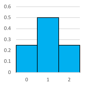
- The number of heads rolled in a set (a set consisting of two coins being flipped) is either 0, 1 or 2. This is represented on the horizontal x-axis.
- The probability of rolling that number of heads in a set is represented on the vertical y-axis.
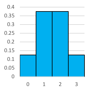
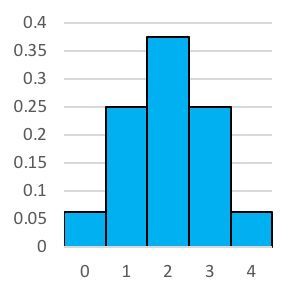
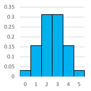
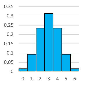
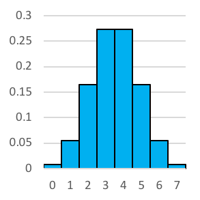
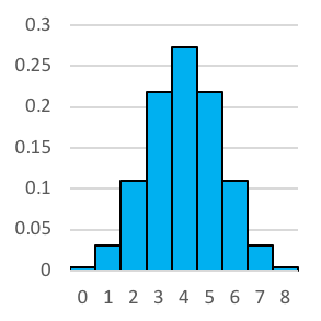
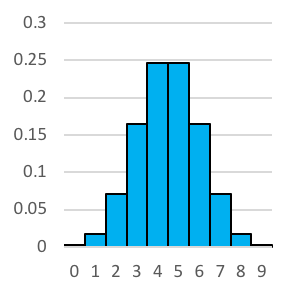
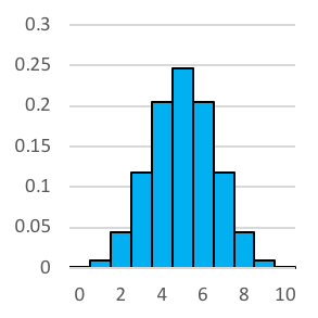
Let’s have a look at what the histograms look like when we increase the number of coin tosses. Reading left to right, we have 2 coin tosses, 3 tosses, 4 tosses and so on until we reach 10 tosses. You’ll no doubt notice that it looks a whole lot like the normal distribution.
 |
 |
 |
 |
 |
 |
 |
 |
 |
Knowing these kinds of distributions is handy when we’re playing games of chance (backgammon anyone?). However, it’s truly incredible how often these kinds of normal distribution patterns occur when we measure things in everyday life.
A reasonable conjecture as to why we observe these kinds of distributions in real life then, is because the myriad of factors that go into a woman’s height or the length of a leaf can be broken down into multiple small probability outcomes that in the end will determine the ultimate characteristic. For example, at a very basic level, we might consider the height of the mother and the height of the father, if both parents are tall, is like tossing two heads on a coin.
Check out this video of a fields medalist who loves the normal distribution.
We can use the normal model as a basis for comparison.
One of the most useful things about the normal model is that we can use it as a basis for comparing results with respect to different variables using a common measure. For example, what is more unusual, a 6m long great white shark or a 5m long saltwater crocodile? If by unusual we mean how rarely it seems to occur, then we need to estimate the distribution of lengths of each of the species.
Suppose the crocodile lengths follow a normal distribution given by N(4.8, 0.3) and the shark lengths follow the model N(5.5, 0.5), we can use these values to determine our expectation of seeing the individuals of these lengths.
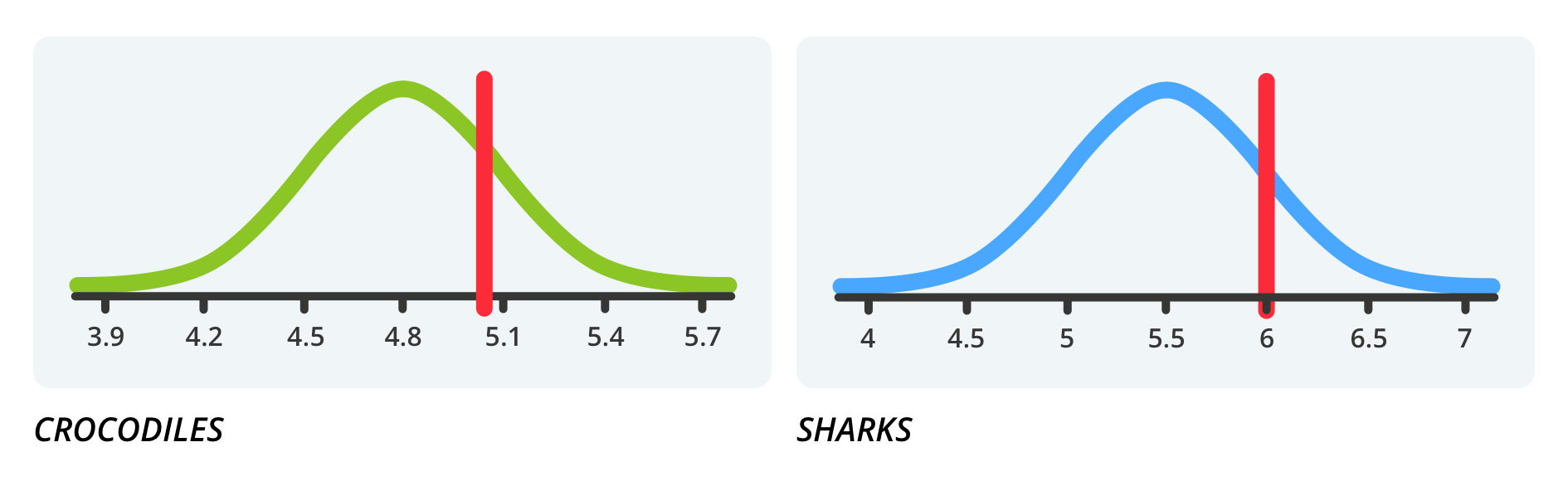
We can see from the position of the 5m crocodile with respect to it’s normal model that perhaps it is less strange than the 6m shark, which sits a whole standard deviation above the mean, whereas the crocodile is less than a whole standard deviation above the mean.
