44 The normal distribution

You’ve probably heard of the bell curve, right?

The normal distribution (also referred to as the “bell curve” or the Gaussian distribution) is a model for the likelihood of observations (i.e. if you go out and collect data). When data follows a normal distribution, there are more observations densely packed towards the centre, and the further away from this centre you get, the rarer the observations. The exact mathematical model that describes this distribution can be attributed to developments by a number of mathematicians including DeMoivre, Laplace, Adrain and Gauss, although it is usually seen as Gauss’s model (hence “Gaussian” distribution). In the last 200 years it has become paramount as a fundamental model in statistics.

Transcript

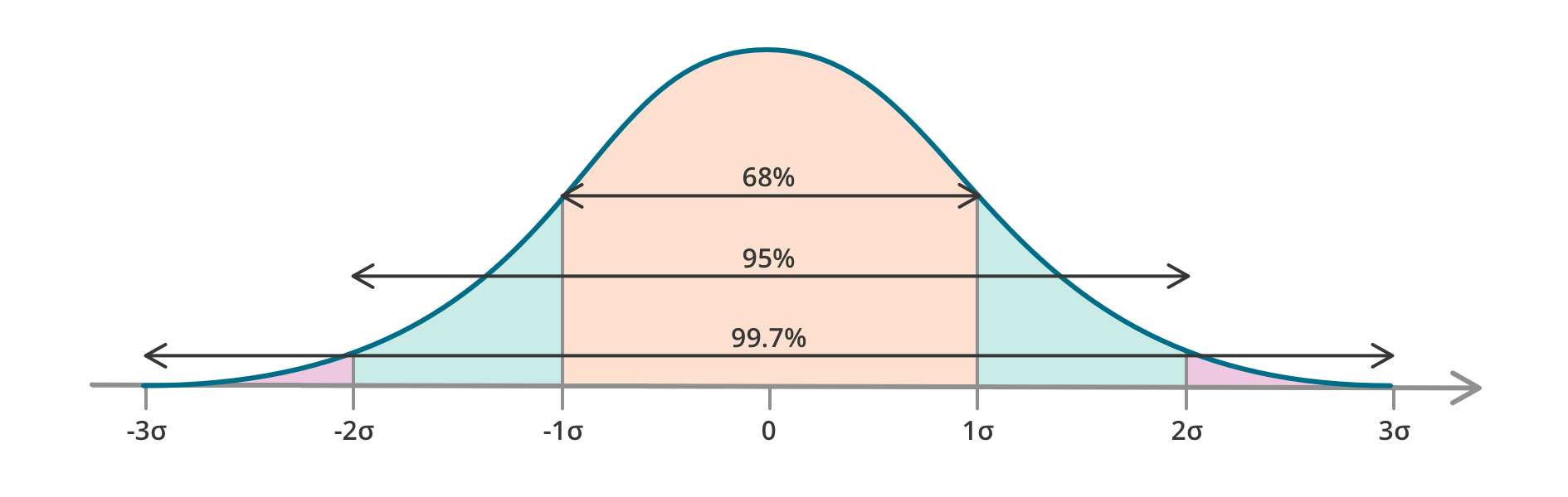
The diagram below summarises the percentages of observations we expect if we have a mean of 0. Sigma (σ) is the mathematical symbol that’s used to represent the standard deviation variable.

The bell curve makes use of the concepts of the mean, and the standard deviation from the mean.

Mean

Finding the mean is simply a matter of adding all the observations together, and then dividing it by the number of observations.  For example, imagine we wanted to find out the mean length of leaves of a particular tree.   We might pick 100 leaves, measure each leaf in mm, add all these measurements together and then divide it by the number of leaves we picked.  It’d look something like this:

[latex]mean \ leaf \ length=\frac{21mm+17mm+20mm... }{100}[/latex]

Standard deviation

Standard deviation is complex to calculate, and you don’t need to be able to do it to follow along in this book.

For now, it’s enough to know that standard deviation is a measure of the average difference of each observation to the mean.   In our tree leaf example, it tells us how likely it is that we will find a tree that’s different or similar to the mean.  This is assuming – and this may be a big assumption – that the length of leaves on the tree follows the normal distribution (if it does, it should look a little bit like a bell curve if we plot it on a histogram).

If a quantity, such as the length of leaves on a tree, does follow a normal distribution, then:

• 68% of observations (leaf length measurements) will be within one standard deviation of the centre (that is, the mean);
• 95% of observations will be within two standard deviations of the centre; and
• 99.7% of observations will be within three standard deviations of the centre.

Let’s take another example.  Let’s consider heights of women. Suppose the average height of an Australian female adult is 162cm with a standard deviation of 7cm. Then we expect 68% of the population to be between 155 and 169cm tall (162 – 7 and 162 + 7), we expect 95% of the population to be between 148 and 176cm tall, and 99.7% of the population to be between 141 and 183cm tall.

We can align this with our probability thinking. If we randomly select a woman from the population, there’s a high chance she’ll be between 155 and 169cm. It’s only in 0.3% of cases (or a 3/1000 chance) that we’d randomly choose someone that’s above 181cm or below 141cm.

Let’s have a go at using the normal distribution model to make predications about the probability of something occurring.

Exercises

Suppose the average height of an Australian woman is 162cm with a standard deviation of 7cm. Suppose, then, that two women were randomly selected from the Australian population. What is the probability that one of them will be below 141cm tall and the other one will be above 183cm tall?