15 Simple Linear Regression
Learning Outcomes
At the end of this chapter you should be able to:
- understand the concept of simple linear regression;
- fit a linear regression model to data in R;
- interpret the results of regression analysis;
- perform model diagnostics;
- evaluate models.
Contents
15.2 Parameter Estimation — Method of Least Squares
15.3 Partitioning the sum of squares
15.8 Outliers and points of high leverage
15.10 Detailed analysis of Beetle data
15.1 Introduction
Many situations require an assessment of which of the available variables affect a particular response or output.
Example 15.1 Case Study: Nelson beetle data
Nelson (1964) investigate the effects of starvation and humidity on weight loss in flour beetle. The data consists of the variables Weightloss (mg) and Humidity (%).
Objective: To quantify the relationship between Weightloss and Humidity.
Reference: Nelson, V. E. (1964). The effects of starvation and humidity on water content in Tribolium confusum Duval (Coleoptera). PhD Thesis, University of Colorado.
Regression is the study of relationships between variables, and is a very important statistical tool because of its wide applicability. Simple linear regression involves only two variables:
![]() independent or explanatory variable;
independent or explanatory variable;
![]() dependent or response variable;
dependent or response variable;
The Model
![]()
where ![]() is the mean of
is the mean of ![]() and
and ![]() is the random variation term. Linear regression assumes that
is the random variation term. Linear regression assumes that ![]() is a linear function of
is a linear function of ![]() , that is
, that is
![]()
THE MODEL
![]()
where
![]() response (or dependent) variable,
response (or dependent) variable,
![]() explanatory (or independent) variable,
explanatory (or independent) variable,
![]() intercept,
intercept,
![]() slope,
slope,
![]() = error or random variation.
= error or random variation.
Model assumptions
Observed data ![]() , and
, and
![]()
We treat ![]() as random variables corresponding to observations
as random variables corresponding to observations ![]() .
.
ASSUMPTIONS
- A linear model is appropriate, that is,
 .
. - The error terms
 are normally distributed.
 - The error terms
 have constant variance.
 - The error terms
 are uncorrelated.
Variance
Note that
![]()
But ![]() is a constant, so
is a constant, so
![]()
assumed constant (that is, ![]() does not depend on
does not depend on ![]() ). The assumptions then imply that
). The assumptions then imply that
![]()
Further,
![]()
since ![]() . This implies that
. This implies that
![]()
15.2 Parameter Estimation — Method of Least Squares
The model has three parameters, ![]() and
and ![]() , and these need to be estimated from the data. Denote by
, and these need to be estimated from the data. Denote by ![]() and
and ![]() respectively the estimates of
respectively the estimates of ![]() and
and ![]() .
.

We use the method of least squares to estimate ![]() and
and ![]() so as to minimise
so as to minimise ![]() .
.
Recall
 is a minimum when
  , from Chapter 2.
 is a minimum when
  .
. .
.
![Rendered by QuickLaTeX.com \begin{align*} \sum_{i=1}^n r_i^2 &= \sum_{i=1}^n \left[Y_i-(B_0+B_1 X_i)\right]^2\\ &= \sum_{i=1}^n \left[(Y_i-B_1 X_i) - B_0\right]^2 \end{align*}](https://oercollective.caul.edu.au/app/uploads/quicklatex/quicklatex.com-fbc44938991b67d551c176d94cc7a36b_l3.png)
![Rendered by QuickLaTeX.com \begin{align*} \sum_{i=1}^n r_i^2 &= \sum_{i=1}^n \left[Y_i-(\overline Y -B_1 \overline X)\right]^2\\ &= \sum_{i=1}^n \left[(Y_i- \overline Y) - B_1(X_i - \overline X)]^2 \end{align*}](https://oercollective.caul.edu.au/app/uploads/quicklatex/quicklatex.com-b442dce1d8542a568f53fd527c77e46b_l3.png)
![Rendered by QuickLaTeX.com \[r_i^2= \sum_{i=1}^n\left(Y_i-\overline Y\right)^2 -2B_1 \sum_{i=1}^n\left(X_i-\overline X\right)\left(Y_i- \overline Y\right)+ B_1^2\sum_{i=1}^n\left(X_i-\overline X\right).\]](https://oercollective.caul.edu.au/app/uploads/quicklatex/quicklatex.com-d1447d0504d627456c2faed8d76a443a_l3.png)
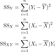
![]()
Now the quadratic function ![]() has a minimum when
has a minimum when ![]() . So this is a quadratic function in
. So this is a quadratic function in ![]() , and has a minimum at
, and has a minimum at ![]() .
.
Thus the least squares estimates of the slope and intercept parameters are:
![]()
Exercise
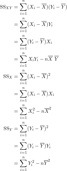
Note
![]()
That is, the point ![]() satisfies the equation of regression, i.e.,
satisfies the equation of regression, i.e., ![]() ALWAYS lies on the line of regression.
ALWAYS lies on the line of regression.
Example 15.3 Beetle data
Nine beetles were used in an experiment to determine the effects of starvation and humidity on water loss in flour beetle. here ![]() = Humidity,
= Humidity, ![]() = Weight.
= Weight.
Summary statistics
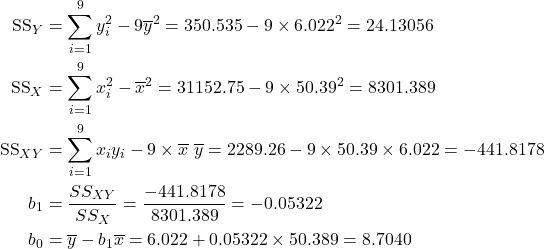
![]()
![]() Estimated average Weightloss for a given humidity
Estimated average Weightloss for a given humidity
Intercept ![]() Average Weightloss when Humidity is zero.
Average Weightloss when Humidity is zero.
Slope ![]() If Humidity increases by 1 % then Weightloss decreases by 0.05322 mg.
If Humidity increases by 1 % then Weightloss decreases by 0.05322 mg.
That is, the beetles prefer a more humid environment in which the weightloss is lower.
15.3 Partitioning the sum of squares
![]()
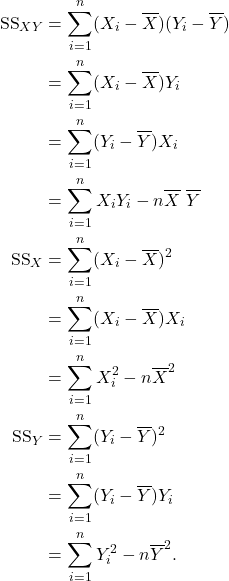
![]()
![]()
Notes
- The SS Reg can also be expressed as follows.
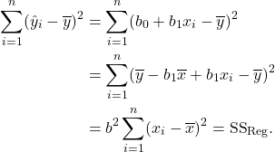
- The proportion of variation explained by the regression is
![Rendered by QuickLaTeX.com \[R^2=\dfrac{\text{SS}_{\text{Reg}}}{\text{SS}_{\text{Total}}}.\]](https://oercollective.caul.edu.au/app/uploads/quicklatex/quicklatex.com-96f3196969cec0da03e3342f788b372f_l3.png)
Note
 .
.
15.4 Hypothesis Test for 
To determine if there is a significant linear relationship between ![]() and
and ![]() , we test the hypotheses:
, we test the hypotheses:

If ![]() is true then
is true then ![]() , so
, so
![]()
Thus we can use the ratio ![]() as a test statistic. However, each of these sums of squares need to be adjusted by their degrees of freedom.
as a test statistic. However, each of these sums of squares need to be adjusted by their degrees of freedom.
![Rendered by QuickLaTeX.com \begin{align*} \text{Regression df} &= \text{Number of parameters -1} \\ &=k-1 =1 \; \text{for simple linear regression}.\\ \text{Total df} &= n-1 \\[12pt] \text{Residual df} &= n-k \\ &= n-2 \; \text{for simple linear regression}. \end{align*}](https://oercollective.caul.edu.au/app/uploads/quicklatex/quicklatex.com-bc49122fee6b77e9da39723e9bedda82_l3.png)
Note that two parameters are estimated from the data in simple linear regression, the intercept and the slope, so ![]() . These calculations can be set up as a table.
. These calculations can be set up as a table.
ANOVA Table
| Source | df | SS | MS | F |
|---|---|---|---|---|
| Regression |
|
|
|
|
| Residual |
|
|
||
| Total |
|
|
The test then proceeds as usual.
If p-value ![]() , where
, where ![]() , then reject
, then reject ![]() , and conclude there is a significant linear relationship between
, and conclude there is a significant linear relationship between ![]() and
and ![]() .
.
Example 15.4 Beetle data (ctd)
![]()
The ANOVA table is given below. Note that the relationships in the ANOVA table are as in chapter 15. That is,
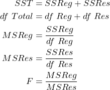
| Source | df | SS | MS | F |
|---|---|---|---|---|
| Regression | 1 | 23.51449 | 23.51449 | 267.18 |
| Residual | 7 | 0.61607 | 0.088010 | |
| Total | 8 | 24.13056 |
The hypothesis of interest are:
![]()
p-value ![]() , so there is overwhelming evidence against the null hypothesis.
, so there is overwhelming evidence against the null hypothesis.
pf(267.18, 1, 7, lower.tail = F)
[1] 7.816436e-07
We conclude based on the linear regression analysis that there is a significant linear relationship between Weightloss and Humidity.
We could also conduct a left-sided test of hypothesis.
![]()
Now the p-value is simply half of the two-sided test. That is,
![]()
so there is overwhelming evidence against the null hypothesis. We conclude based on the linear regression analysis that there is a significant negative linear relationship between Weightloss and Humidity.
15.5 Estimate of 
The final model parameter that needs to be estimated is the constant error variance term ![]() . Now
. Now
![]()
which can be estimated by the average of the residuals squared. That is,
![]()
Note that here we have used the data to estimate ![]() parameters/regression coefficients. For simple linear regression,
parameters/regression coefficients. For simple linear regression, ![]() . Also note that as in ANOVA,
. Also note that as in ANOVA,
![]()
which can be read from the ANOVA table for regression.
For the Beetle data, ![]() .
.
15.6 Distribution of 
![]()
The random variables here are ![]() , and
, and ![]() are considered constant. Put
are considered constant. Put
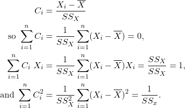
Then
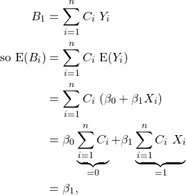
so ![]() is an unbiased estimator of
is an unbiased estimator of ![]() .
.
Next,
![]()
Further, ![]() are normally distributed, so
are normally distributed, so ![]() is the sum of normal random variables; thus
is the sum of normal random variables; thus ![]() is also normal.
is also normal.

If ![]() is unknown (usually the case), we replace it by
is unknown (usually the case), we replace it by ![]() , and then
, and then

We can thus use the t-distribution for (one-sided and two-sided) hypothesis tests and confidence intervals for ![]() .
.
Example 15.4 Beetle data
![]()
Is there a significant
- linear relationship
- positive linear relationship
between Sales and Promotions
Solution
The hypothesis are ![]() against the two-sided
against the two-sided ![]() or the right-sided
or the right-sided ![]() .
.
Test statistic is

- The two-sided p-value
 so there is overwhelming evidence against the null hypothesis. Same p-value and conclusion as before.
 - One-sided test. p-value
 so there is overwhelming evidence against the null hypothesis. Same p-value and conclusion as before.
Note
- The p-values from the F-distribution and the t-distribution are the same here. Note that
![Rendered by QuickLaTeX.com \[(t_{obs})^2 = (-16.34563)^2 = 267.1796 = F_{obs}\]](https://oercollective.caul.edu.au/app/uploads/quicklatex/quicklatex.com-1270df1d962da8f9bc67f1f8b6c7b15d_l3.png)
from the ANOVA table. In fact
![Rendered by QuickLaTeX.com \[(t_k)^2 = F_{1,k}.\]](https://oercollective.caul.edu.au/app/uploads/quicklatex/quicklatex.com-602fc733ca99969013108546b780ef85_l3.png)
- The one-sided p-value is simply half the two-sided p-value from either the t- or F-distribution.
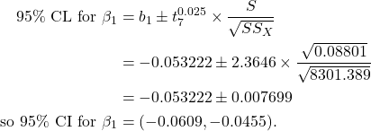
Example 15.4 Beetle data –Confidence interval
A 95% confidence interval for ![]() is calculated as before.
is calculated as before.
15.7 Model diagnostics
Model assumptions are verified by analysis of residuals. There are four assumptions.
- A linear model is appropriate.
- Scatterplot of
 against
  . This should show points roughly around a straight line. This is usually part of the data exploration before model fitting.
 - Scatterplot of standardised residuals against fitted values. The plot should be patternless. This is the best plot to verify this assumption, and is also used in the next chapter on multiple regression.
- Scatterplot of standardised residuals against
 . Plot should be without pattern. This is similar to the previous plot. It is also used in the next chapter on multiple regression for model building and selecting if some transformation of data is appropriate.
- Scatterplot of
- The errors are normally distributed. These are verified as for ANOVA.
- Histogram of residuals.
- Normal probability plot.
- Chi-squared test of normality. We won’t cover this.
- Errors have constant variance. This is again by inspecting residual plots, as for ANOVA.
- Plot of standardised residuals against fitted values. Should have constant spread. This is the best plot and is also used in the next chapter on multiple regression.
- Plot of standardised residuals against
 . Should have constant spread. In the case of multiple regression this plot may help identify variables that are related to inhomogeneous variance.
- Errors are uncorrelated. Durbin–Watson test statistic. This is beyond the scope of this text.
Example 15.5 (a)
Evaluate the model with the given diagnostic plots.
Solution
The scatterplot appears close to a straight line, and the plot of residuals against fitted values shows no clear pattern, so a linear model is appropriate. The histogram of residuals is not too different from that expected for a normal distribution, showing only a light asymmetry, and the normal probability plot does not depart markedly from a straight line. We conclude that the normality assumption is not violated. Finally, the plot of residuals against fitted values shows no change in spread, so there is no evidence against the homogeneous variance assumption.
Example 15.5 (b)
Solution
Evaluate the model with the given diagnostic plots.
Solution
The plot of residuals against fitted values shows a quadratic trend, so a linear model is not appropriate. The departure from normality is also evident from the histogram and normal probability plot, but this may be due to the linear model not being appropriate. The homogeneous variance assumption seems to be satisfied as there is no change in spread in the plot of residuals against fitted values.
Example 15.5 (c)
Evaluate the model with the given diagnostic plots.
Solution
The plot of residuals against fitted values indicates a “fanning out”, so the homogeneous variance assumptions is violated. A linear model seems appropriate and there is no evidence against the normality assumption.
Example 15.5 (d)
Evaluate the model with the given diagnostic plots.
Solution
From the histogram and normal probability plot, it is clear that the normality assumption does not hold. The scatterplot of the data indicates that a linear model may not be appropriate. Similarly the plot of residuals against fitted values shows evidence against the homogeneous variance assumption. However, these issues may be due to a lack of normality.
15.8 Outliers and Points of High Leverage
Outliers are points away from the bulk of the data. They usually have large absolute residuals, that is, large positive or large negative residuals, and are easily identified from plots. Commonly ![]() is used to identify outliers.
is used to identify outliers.
Outliers are important because they may affect model fit. To investigate the effect of an outlier the regression model should be fitted with and without the point for comparison.
If in arriving at the final model any outliers have been omitted then this should be reported. One should never silently omit outliers. Indeed, if enough points are omitted then one can arrive at a perfect model.
Points of high leverage are those that strongly influence the goodness of fit of the model. These usually have small absolute residuals, close to zero. Again the model should be fitted with and without them.
The graph above shows a point that is away from the bulk of the data. This point is an outlier. It is also a point of high leverage, since the linear model is very strongly influenced by it. Removing it and re-fitting the model gives the graph below. This plot shows there really is no model between the variables here.
15.9 Correlation coefficient
The correlation coefficient, ![]() , is a measure of the strength of the linear relationship between
, is a measure of the strength of the linear relationship between ![]() and
and ![]() .
.
![]()
Then
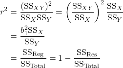
Note that ![]() , so
, so ![]() .
.
![]()
and ![]()
and ![]() , so the points
, so the points ![]() lie on a straight line.
lie on a straight line.
If ![]() is close to 1, then a strong linear relationship exists between
is close to 1, then a strong linear relationship exists between ![]() and
and ![]() .
.
If ![]() is close to 0, no linear relationship exists between
is close to 0, no linear relationship exists between ![]() and
and ![]() .
.
Note that
![]()
so ![]() has the same sign as
has the same sign as ![]() . Testing
. Testing ![]() is equivalent to testing
is equivalent to testing ![]()
CAUTION
![]() large means a strong linear relationship exists between
large means a strong linear relationship exists between ![]() and
and ![]() . It DOES NOT mean “
. It DOES NOT mean “![]() causes
causes ![]() ”. It is possible that
”. It is possible that ![]() and
and ![]() are both related through a third variable. Spurious correlation is often misused to imply causation.
are both related through a third variable. Spurious correlation is often misused to imply causation.
If ![]() is small, it does not indicate that
is small, it does not indicate that ![]() and
and ![]() are unrelated — it only indicates a lack of a linear relationship.
are unrelated — it only indicates a lack of a linear relationship. ![]() and
and ![]() may still be related non-linearly.
may still be related non-linearly.
If we reject ![]() , then there is a significant linear relationship between
, then there is a significant linear relationship between ![]() and
and ![]() . This DOES NOT indicate that the relationship is a good one, or the best one. Residual analysis should be performed to verify model assumptions. A similar comment applies if
. This DOES NOT indicate that the relationship is a good one, or the best one. Residual analysis should be performed to verify model assumptions. A similar comment applies if ![]() is large.
is large.
Example 15.6 Example of weak correlation but strong relationship
The scatterplot shows a very strong non-linear relationship between ![]() and
and ![]() , but a zero correlation.
, but a zero correlation.
ALWAYS examine a plot of the data!
15.10 Detailed analysis of the Beetle data: with R code
The data consists of observations for nine beetles for the variables Weightloss (mg) and Humidity (%).
Objective: To quantify the relationship between sales and promotional expenses.
The figure below shows a scatterplot of the data and some summary statistics.
> nelson<-read.csv("nelson.csv", header=T)
 Humidity       Weightloss
 Min.   : 0.00   Min.   :3.720
 1st Qu.:29.50   1st Qu.:4.680
 Median :53.00   Median :5.900
 Mean   :50.39   Mean   :6.022
 3rd Qu.:75.50   3rd Qu.:6.670
 Max.   :93.00   Max.   :8.980
 sd     : 32.21  sd     :1.74
> with(nelson, plot(Weightloss ~ Humidity))
Observations
The data range for Humidity is 0–93, with mean 50.39 and median 53.00. Weightloss has a range of 3.272–8.98, with mean 6.022 and median 5.900.
The scatter plot shows that a linear relationship is feasible.
Note that the function to fit the regression model is lm(). The ANOVA table is given, as well as a table of coefficients, standard errors for the coefficients and the p-values.
The output of the regression analysis in R is given below. The function to fit the linear model is lm().
> nelson.lm<-lm(Weightloss ~ Humidity, data = nelson)# y ~ x is the model formula,
#and the dataframe is specified by data = nelson.
> summary(nelson.lm)

Call:
lm(formula = Weightloss ~ Humidity, data = nelson)

Residuals:
     Min       1Q   Median       3Q      Max
-0.46397 -0.03437  0.01675  0.07464  0.45236

Coefficients:
             Estimate Std. Error t value Pr(>|t|)
(Intercept)  8.704027   0.191565   45.44 6.54e-10 ***
Humidity    -0.053222   0.003256  -16.35 7.82e-07 ***
---
Signif. codes:  0 ‘***’ 0.001 ‘**’ 0.01 ‘*’ 0.05 ‘.’ 0.1 ‘ ’ 1

Residual standard error: 0.2967 on 7 degrees of freedom
Multiple R-squared:  0.9745,	Adjusted R-squared:  0.9708
F-statistic: 267.2 on 1 and 7 DF,  p-value: 7.816e-07
The coefficients of the model are given, along with the corresponding standard errors and p-values. The output below the coefficient table gives the residual standard error, which is the estimate of the model standard deviation ![]() . The degrees of freedom of th residual standard error is also given. It also gives the value of the correlation coefficient squared. Finally, the F-value, its corresponding degrees of freedom and p-value are also given.
. The degrees of freedom of th residual standard error is also given. It also gives the value of the correlation coefficient squared. Finally, the F-value, its corresponding degrees of freedom and p-value are also given.
We will discuss the other output in the next chapter. Here we will calculate the Multiple R-Squared and Adjusted R-squared.
The adjusted R-squared and Adjusted R-squared are defined as
![]()
and

where ![]() number of observations and
number of observations and ![]() number of variables.
number of variables.
The calculations in R are below.
(SST <- sum(anova(nelson.lm)[2]))
[1] 24.1306
> (SSRes <- anova(nelson.lm)[2][[1]][2])
[1] 0.616063
> (Rsq <- 1-SSRes/SST)
[1] 0.97447
> (Totdf <- sum(anova(nelson.lm)[1]))
[1] 8
> (Resdf <- (anova(nelson.lm)[1][[1]][2]))
[1] 7
> (AdjRsq <- 1- (SSRes/Resdf)/(SST/Totdf))
[1] 0.970822
Scatterplot of Beetle data is given below, with regression line superimposed. The equation of the line and the correlation coefficient is also stated.
Two and one sided hypothesis tests for ![]() can be conducted using the output.
can be conducted using the output.
![]()
For the coefficient for Humidity, the one-sided p-value ![]() . At the 2.5% level of significance we will reject the null hypothesis and conclude that a strong linear relationship exists between Weightloss and Humidity.
. At the 2.5% level of significance we will reject the null hypothesis and conclude that a strong linear relationship exists between Weightloss and Humidity.
Confidence Intervals can be easily obtained. Compare this with the calculation in Example 15.4.
confint(nelson.lm)
                  2.5 %      97.5 %
(Intercept)  8.25104923  9.15700538
Humidity    -0.06092143 -0.04552287
The ANOVA table for the regression is given below.
> anova(nelson.lm)
Analysis of Variance Table

Response: Weightloss
          Df  Sum Sq Mean Sq F value    Pr(>F)
Humidity   1 23.5145  23.515  267.18 7.816e-07 ***
Residuals  7  0.6161   0.088
Compare the ANOVA table values with those given in the regression output. The F-value, degrees of freedom and p-values are the same as in the regression output. Note that the square root of the Residual mean sum of squares,
![]()
which is equal to the residual standard error from the linear regression output.
The figure below may be used to verify the assumptions of linear regression.
> oldpar<-par(mfrow=c(2,2)) #mfrow (multi figure row) specifies the number of rows
# and columns the plots should be arranged in.
> nelson.res<-rstandard(nelson.lm)
> hist(nelson.res,xlab="Standardised residuals", ylab="Frequency")
> box()
> plot(nelson.res~nelson.lm$fitted.values, xlab="Fitted values",
ylab="Standardised residuals",main="Standardised residuals vs Fitted")
> qqnorm(nelson.res,xlab="Normal scores", ylab="Standardised residuals")
> par(oldpar)
-
A linear model is appropriate. The plot of standardised residuals against predicted Sales and Promotions shows noobvious pattern, so we conclude that a linear model is appropriate.
- Residuals are normal. We have only nine observations so normality cannot be verified. Nonetheless, the normal probability plot is not too far from a straight line. Additionally, the histogram shows a plot that is not too different to that expected for a normal distribution, despite the gaps. We conclude that there is no evidence against the normality assumption.
- Residuals have a constant variance. The plot of standardised residuals against predicted Weightloss seems to indicate some “fanning” outward, but this is perception is due to the small sample size.
Note that there are no outliers in the data since the standardised residuals are all between ![]() and
and ![]() .
.
5.11 Prediction
Predictions can be made using the predict function in R . This is easy to use – check the online help in you are unsure. For example, to forecast the Weightloss for Humidity = 1, 2, 3, 4, 5, and 6:
new=data.frame(Humidity=c(1:6))
> predict(nelson.lm,new)
       1        2        3        4        5        6
8.650805 8.597583 8.544361 8.491139 8.437917 8.384694
15.12 Warning: Always perform model diagnostics
Given below is the output of a regression analysis.
Call:
lm(formula = y ~ x)

Residuals:
   Min     1Q Median     3Q    Max
 -10.0   -7.5   -1.0    6.0   15.0

Coefficients:
            Estimate Std. Error t value Pr(>|t|)
(Intercept) -15.0000     5.5076  -2.724   0.0235 *
x            10.0000     0.9309  10.742 1.97e-06 ***
---
Signif. codes:  0 ‘***’ 0.001 ‘**’ 0.01 ‘*’ 0.05 ‘.’ 0.1 ‘ ’ 1

Residual standard error: 9.764 on 9 degrees of freedom
Multiple R-squared:  0.9276,	Adjusted R-squared:  0.9196
F-statistic: 115.4 on 1 and 9 DF,  p-value: 1.967e-06
Observations
- The coefficient of determination is 0.9740, so about 97% of the variation in the data is explained by the regression. The p-value is
 , so there is a significant linear relationship between the variables.
 - This does not mean that the linear regression is a good one. We have not performed any model diagnostics yet. In particular, we do not even know that a linear model is even appropriate! It is very important to perform some EDA before the regression analysis.
The scatter plot of the data shows that there is a problem with the linear model — the data points follow a pattern. This is much more clear in the plot of residuals against predicted values and x values. (This is the reason for residual plots — any patterns are accentuated). Both show that a quadratic model is appropriate. In fact the data comes from ![]() , as you can check from the scatter plot of the data.
, as you can check from the scatter plot of the data.
This example clearly shows that just the Anova, correlation coefficient and hypothesis test are not enough to justify a linear model.
15.13 A note on outliers
Outliers usually lead to model misfit and are commonly omitted. However, outliers are still part of the data. It is important to understand the reasons for the outliers. These points should be investigated to see how they differ from the rest of the data. What are the particular characteristics of outliers? Do they, for example, represent observations from a sub-population with some special features?
As an example, if a clinical trial is conducted for a drug for weight loss, and it is found that out of a sample of size 500, ten people have sharp abdominal pains. Are these outliers and should they be ignored or omitted? In this case it is important to investigate these ten people further to understand if they have any particular characteristics that may explain the pain. If for example all ten are females over 50, then a very strong caveat for the drug needs to be that females over 50 should not be taking this drug.
If these ten points are omitted and simply ignored, then when the sample is generalised to an entire population the ten people are scaled to several hundred thousand to millions, and this is a serious medical problem.
15.14 Summary
- State the linear regression model and explain the meaning of each term.
- Fit a linear regression model in R and interpret the output.
- Understand the Anova table for regression.
- Perform a test of hypothesis for the slope parameter
 using either the F-distribution or the t-distribution in the R output.
 - Find confidence intervals for the slope parameter.
- Predict the values of y from the fitted equation for regression.
- Know when the prediction is reliable.
- Know some simple relationships between sums of squares, degrees of freedom and the coefficients of regression.

