14 ANOVA
Learning Outcomes
At the end of this chapter you should be able to:
- state the hypotheses for ANOVA;
- obtain an ANOVA table given summary statistics;
- perform a test of hypothesis for ANOVA;
- compute the estimate of variance;
- verify assumptions for the models used in the hypothesis tests;
- compute confidence intervals for a single mean and a difference of means;
- perform a Kramer-Tukey multiple comparison analysis and interpret the results.
Contents
14.1 Introduction
14.2 Hypotheses
14.3 Model equation
14.4 Partitioning the sum of squares
14.5 The ANOVA Table
14.6 Model assumptions
14.7 Estimate of 
14.8 Confidence intervals
14.9 Multiple comparisons
14.10 Summary
14.1 Introduction
In Chapter 13.2 we considered two independent samples from two populations with respective means  and
and  . We now extend this to
  independent samples from populations with means
  . This is a common situation. It is unwise to start by comparing every possible pair of populations using two-sample tests because:
- it is a lot of work. For example, there are more than 100 pairwise comparisons between 15 samples.
- problems with significance levels in multiple testing.
ANOVA data often arise from designed experiments.
Example 14.1 Toxicology experiments
Many toxicological experiments compare the impact of chemical compounds in the diets of rats. Forty rats were randomly assigned to one of 4 treatments groups. The treatment groups are control, low, medium, high levels of a chemical compound in their diet. At the end of the experiment the rats were euthanised and every organ in the body was weighed. The question of interest is to determine whether the diet of the rats has an impact on the weight of organs (for instance liver weight).
Example 14.2 Discrimination Against People with Disability
Researchers prepared 5 videotaped job interviews using actors with a script designed to reflect an interview with an applicant of average qualifications. The 5 tapes differed only in that the applicant appeared with a different disability in each one. Seventy undergraduate students were randomly assigned to view the tapes. The researchers were required to rate the qualification of the applicant on a 0-10 point scale.
Example 14.3 Zinc diatom species
Medley and Clements (1998) studied the impact of zinc contamination (and other heavy metals) on the diversity of diatomic species in Rocky Mountains, USA. The level of zinc contamination (background, high, medium and low) and diversity of diatoms (number of species) were recorded from between four and six sampling stations within each of six streams known to be polluted. Does the level of zinc contamination affect the diversity of diatom species in the Rocky Mountains?
Reference: Medley, C. N. and Clements, W. H. (1998) Reponses of diatom communities to heavy metals in streams: The influence of longitudinal variation. Ecological Applications, Vol 8, No. 3, pp631–644.
ANOVA compared to the two-sample t-test
In Chapter 13 we carried out a two-sample t-test on the SIRDS data. We assumed equal variance.
ttest <- t.test(survived, died, var.equal = TRUE)

	Two Sample t-test

data:  survived and died
t = 2.0929, df = 24, p-value = 0.04711
alternative hypothesis: true difference in means is not equal to 0
95 percent confidence interval:
 0.007461898 1.071228578
sample estimates:
mean of x mean of y
 2.267917  1.728571
- The
 value is 2.0929.
 - The degrees of freedom for this test are 24 (
 ).
). - The p-value for the test of difference in two means was 0.04711.
- We assumed that the two populations that the samples were from had the same variance.
- A 95% confidence interval for a difference in means is
 .
.
Next we run Bartlett’s test for equality of variance.
survived <- c(1.130,1.680,1.930,2.090,2.700,3.160,3.640,1.410,1.720,2.200,2.550,3.005)
died <- c(1.050,1.230,1.500,1.720,1.770,2.500,1.100,1.225,1.295,1.550,1.890,2.200,2.440,2.730)
Status <- c(rep(c("Survived"), 12), rep(c("Died"), 14))
Weight <- c(survived, died)
sirds <- data.frame(Status, Weight)
tapply(sirds$Weight, sirds$Status, mean)
    Died Survived
1.728571 2.267917
tapply(sirds$Weight, sirds$Status, sd)
     Died  Survived
0.5535912 0.7576982
t.test(Weight ~ Status, var.equal = TRUE) #Another way of performing t-test, using a model formula.

	Two Sample t-test

data:  Weight by Status
t = -2.093, df = 24, p-value = 0.0471
alternative hypothesis: true difference in means between group Died and group Survived is not equal to 0
95 percent confidence interval:
 -1.0712286 -0.0074619
sample estimates:
    mean in group Died mean in group Survived
               1.72857                2.26792
bartlett.test(Weight ~ Status, data = sirds)
Bartlett test of homogeneity of variances data:
Weight by Status Bartlett's K-squared = 1.1277, df = 1, p-value = 0.2883
Have a careful look at the above R script and output. The variances for the died and survived groups are respectively 0.5536 and 0.7577. These do not appear to be different. The Bartlett’s test gives a p-value = 0.2883. The null hypothesis of the test is that the variances are not different, and the alternative hypothesis is that they are. Based on this test we conclude that the variances are not different, so the equal variance assumption is satisfied.
____________________________________________________________________________________________
Reporting on the SIRDS analysis
Reporting on statistical analysis is an important skill. Below we present an example report on the SIRDS analysis.
Method
We used a two independent samples t-test (two sided) assuming equal variance to determine whether there was evidence of a difference in birth weight between SIRDS infants that survived and SIRDS infants that died. We used a 5% significance level and presented a 95% confidence interval for difference in true population means.
Results
There was a statistically significant difference between the mean weight of children who survived and those who died in terms of birth weight (p-value = 0.04711) estimated difference in means 0.53935 kg (survived-died) with a 95% confidence interval (0.00746, 1.72857). Bartlett’s test (p-value = 0.2883) indicated that the equal variance assumption is not violated.
Conclusion
Based on the analysis we conclude there is sufficient evidence to demonstrate a statistically significant difference in mean birth weights of surviving and dead SIRDS infants. The surviving infants have a higher mean birth weight.
__________________________________________________________________________________________
Before we discuss the details of the procedure, we will perform an ANOVA analysis on the SIRDS data in R.
sirds.anova <- aov(Weight ~ Status, data = sirds)
summary(sirds.anova)
            Df Sum Sq Mean Sq F value Pr(>F)
Status       1   1.88  1.8796    4.38 0.0471 *
Residuals   24  10.30  0.4291
Note that the output looks different, but the p-value is the same.
So what is ANOVA?
ANOVA is a powerful technique for comparing the means of two or more populations. The different populations in ANOVA can be defined by one or more factors (i.e. categorical explanatory variables). ANOVA tests for the effect of these factors on the response variable.
Consider the zinc data set of Medley and Clements (1998) in Example 14.3. How do we assess whether there is difference in group means?

The boxplot above shows that HIGH zinc level has lower mean diversity compared with the other levels. Given that there is no overlap of the boxplot for HIGH with the other levels, this difference seems to be significant.
How do we assess difference between the groups statistically? We partition each individual measurement into components, as illustrated in the figure below.
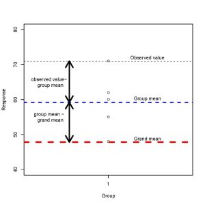
Every observation can be expressed as
observed value = grand mean + (group mean – grand mean) + (observed value – group mean)
We assess whether there is evidence of a difference in groups by looking at these differences between groups and within groups.
The data for ANOVA is as below.
| Population (mean, variance) | Sample (responses) | Mean |
|---|---|---|
| 1 |
|
|
| 2 |
|
|
 |
|
|
|
|
|
![\[y_{11}, y_{12}, \ldots, y_{1n_1}\]](https://oercollective.caul.edu.au/app/uploads/quicklatex/quicklatex.com-594c2b81c9690b4039fc8fb9dcfd4aa1_l3.png "Rendered by QuickLaTeX.com")
![\[\overline y_1\]](https://oercollective.caul.edu.au/app/uploads/quicklatex/quicklatex.com-3facad3e0571fc129284c570d145eceb_l3.png "Rendered by QuickLaTeX.com")
![\[y_{21}, y_{22}, \ldots, y_{2n_2}\]](https://oercollective.caul.edu.au/app/uploads/quicklatex/quicklatex.com-63c0fab2e9eacde0c582e05a5067b709_l3.png "Rendered by QuickLaTeX.com")
![\[\overline y_2\]](https://oercollective.caul.edu.au/app/uploads/quicklatex/quicklatex.com-a2fe2e19500348311c3ce3697a1a3863_l3.png "Rendered by QuickLaTeX.com")
![\[\vdots\]](https://oercollective.caul.edu.au/app/uploads/quicklatex/quicklatex.com-3be7f1152dc60ce277ad506edd3c7915_l3.png "Rendered by QuickLaTeX.com")
![\[y_{k1}, y_{k2}, \ldots, y_{kn_k}\]](https://oercollective.caul.edu.au/app/uploads/quicklatex/quicklatex.com-249ac54c3ba26e05cdbe74b6174842ca_l3.png "Rendered by QuickLaTeX.com")
![\[\overline y_k\]](https://oercollective.caul.edu.au/app/uploads/quicklatex/quicklatex.com-2a1b67ddc983d3bfb3affd4b79d179c0_l3.png "Rendered by QuickLaTeX.com")
We define the grand mean, denoted  , as the mean of all the data (irrespective of which sample they come from). The total number of observations is denoted
  where
where
![\[n=n_1+n_2+\ldots +n_k.\]](https://oercollective.caul.edu.au/app/uploads/quicklatex/quicklatex.com-657cbbecf7f255ffc705ec59e4f3421b_l3.png "Rendered by QuickLaTeX.com")
Assumptions of ANOVA
These assumptions are the same as that for the two independent samples t-test.
- Each sample is from a normally distributed population.
- The observations within each sample are independent, and each sample is independent of the other samples.
- The populations have a common variance (homoscedacity), that is,
![\[\sigma_1^2 = \sigma_2^2 = \ldots = \sigma_k^2 = \sigma^2.\]](https://oercollective.caul.edu.au/app/uploads/quicklatex/quicklatex.com-8d32fad01bb2cd0b2d033c90dc12674b_l3.png "Rendered by QuickLaTeX.com")
14.2 Hypotheses
 (The population means are equal).
 : Not all the means are equal or
  is false.
Evidence for (that is, against ) will be provided by a substantial degree of variability (difference) between the sample means.
14.3 Model equation
Similar to the two independent samples model, the data for ANOVA are:
- Explanatory (or independent variable) which is categorical:
 , represents population
  from which the sample is taken.
 - Response (or dependent variable) which is continuous:
 represents observation
  from sample , where
  is the group/population number and
  .
.
The model equation is
Model Equation
![\[Y_{ij} = \mu_i + \epsilon_{ij},\]](https://oercollective.caul.edu.au/app/uploads/quicklatex/quicklatex.com-24283f91754a4d2637a439bfb29c4b1b_l3.png "Rendered by QuickLaTeX.com")
where  is the random variation (or error) term and
  is the mean of group . The model equation simply states that group has mean .
14.4 Partitioning the sum of squares
We express the observations as
![\[Y_{ij}= \underbrace{\bar Y}_{\mbox{grand mean}} + \underbrace{(\bar Y_i - \bar Y)}_{\mbox{deviation of sample $i$}} + \underbrace{(Y_{ij} - \bar Y_i)}_{\mbox{residual}}\]](https://oercollective.caul.edu.au/app/uploads/quicklatex/quicklatex.com-6e0df08cd6eb740f9276fcb16c67c5b3_l3.png "Rendered by QuickLaTeX.com")
If is correct then  , and hence
  , should be quite close to zero for each sample. It can be shown that

where SS is an abbreviation for `sum of squares’.
Treatment SS
![\[SS_{ttt}=\sum_{i=1}^k n_i (\bar Y_i - \bar Y)^2\]](https://oercollective.caul.edu.au/app/uploads/quicklatex/quicklatex.com-207c062934f904af32987af9f851e0f9_l3.png "Rendered by QuickLaTeX.com")
Treatment SS (also called Between SS, denoted SSB) measures variation between the groups.
If is true, then all the group means should be close to each other, and also close to the grand mean  ; this will cause SSB to be small.
Residual SS
![\begin{align*} SS_{Res}&=\sum_{i=1}^k\sum_{j=1}^{n_i} (Y_{ij} - \bar Y_i)^2\\ &= \sum_{i=1}^k (n_i-1)\left[\frac{1}{n_1-1}\sum_{j=1}^{n_i}(Y_{ij} - \bar Y_i)^2\right]\\ &= \sum_{i=1}^k (n_i-1) s_i^2. \end{align*}](https://oercollective.caul.edu.au/app/uploads/quicklatex/quicklatex.com-4dcf0511a80131a9b592bb1baf9041a2_l3.png "Rendered by QuickLaTeX.com")
Residual SS (also called Within SS, denoted SSW) measures variation within the groups.
Total SS
![\[SS_{tot}=\sum_{i=1}^k \sum_{j=1}^{n_i} (Y_{ij} - \bar Y)^2\]](https://oercollective.caul.edu.au/app/uploads/quicklatex/quicklatex.com-92c7f27a32ee664bfce8f8fb6aa2781a_l3.png "Rendered by QuickLaTeX.com")
Total SS measures the total variation in the data.
If is true, then the variation between groups is small, and the total variation is largely explained by the variation within the groups. Thus the ratio  would be small. But
  is based on only observations while
  is based on . So first we divide each by its degrees of freedom to compute the Mean SS.
The computations can be set up as a table.
14.5 The ANOVA Table
| Source | df | SS | MS | F |
|---|---|---|---|---|
| Treatment |  |
|
|
|
| Residual |  |
 |
|
|
| Total |  |
|
![\[MS_{ttt} = \frac{SS_{ttt}}{k-1}\]](https://oercollective.caul.edu.au/app/uploads/quicklatex/quicklatex.com-d62c4bb19dca180757c114f56219b564_l3.png "Rendered by QuickLaTeX.com")
![\[\frac{MS_{ttt}}{MS_{Res}} \sim F_{k-1, n-k}\]](https://oercollective.caul.edu.au/app/uploads/quicklatex/quicklatex.com-5f7301a344d29c9a94ae3a8ffd7cb630_l3.png "Rendered by QuickLaTeX.com")
![\[MS_{Res} = \frac{SS_{Res}}{n-k}\]](https://oercollective.caul.edu.au/app/uploads/quicklatex/quicklatex.com-518e0d998b520d2ccc452d423fa24501_l3.png "Rendered by QuickLaTeX.com")
Hypothesis test
If the populations truly have different means (i.e. if the factor has a real effect on the responses) then the Factor MS should be relatively large compared to the Error MS. Hence, an appropriate test statistic is
![\[F = \frac{MS_{ttt}}{MS_{Res}}\]](https://oercollective.caul.edu.au/app/uploads/quicklatex/quicklatex.com-de66fd93856fef5c6041af880c5e0f6a_l3.png "Rendered by QuickLaTeX.com")
with extreme positive values of  providing evidence against .
Under the assumption that is correct, has an F-distribution with  degrees of freedom. The P-value for an observed value
  of the F-statistic is
![\[P = P(F \ge f)\]](https://oercollective.caul.edu.au/app/uploads/quicklatex/quicklatex.com-af0ab0b876aca526b5a5ab5370edafb5_l3.png "Rendered by QuickLaTeX.com")
where has the F has an  distribution.

Example 14.4
An orange juice company has four machines that fill two-litre plastic containers with juice. In order to determine if the mean volume filled by these machines is the same, the quality control manager collects a random sample of 19 containers filled by different machines and measures their volumes. The data obtained is given below, along with some summary statistics. What should the manager conclude? Use  . What are the implications of your findings?
| Machine 1 | Machine 2 | Machine 3 | Machine 4 |
|---|---|---|---|
| 2.05 | 1.99 | 1.97 | 2.00 |
| 2.01 | 2.02 | 1.98 | 2.02 |
| 2.02 | 2.01 | 1.97 | 1.99 |
| 2.04 | 1.99 | 1.95 | 2.01 |
| 2.00 | 2.00 | ||
| 2.00 |
Means: 
Grand mean 
Standard deviation: 
Sample size: 
Solution
First we explore the data. A scatterplot of the data is given below. The scatterplot shows that Machine 3 seems to produce the lowest volumes, while Machine 1 produces the highest. Machines 2 and 4 show no apparent difference in volumes. The spread of volumes appears to be equal for all the machines. The above observations are confirmed by the summary statistics given in the table.

The R code for the scatterplot and some summary statistics is given below.
orange<-read.table("orange.txt", header=T, sep="\t", stringsAsFactors = T)
> summary(orange)
    Machine          Volume
 Min.   :1.000   Min.   :1.950
 1st Qu.:1.000   1st Qu.:1.990
 Median :2.000   Median :2.000
 Mean   :2.316   Mean   :2.001
 3rd Qu.:3.000   3rd Qu.:2.015
 Max.   :4.000   Max.   :2.050
> with(orange, tapply(Volume, Machine, mean))
     1      2      3      4
2.0200 2.0020 1.9675 2.0050
> with(orange, tapply(Volume, Machine, sd))
         1          2          3          4
0.02097618 0.01303840 0.01258306 0.01290994
> mean(orange$Volume)
[1] 2.001053
> plot(orange$Volume ~ orange$Machine, xlab = "Machine", ylab = "Volume")
Let be the mean volume of juice from machine ,  . The hypotheses of interest are:

The calculations for the sums of square are given below.

Based on these, the ANOVA table can be constructed. We give the corresponding table from R.
orange.anova<-aov(Volume~Machine, data=orange)
summary(orange.anova)
                Df   Sum Sq  Mean Sq F value  Pr(>F)
factor(Machine)  3 0.006724 0.002241   8.721 0.00137 **
Residuals       15 0.003855 0.000257
Total           18 0.010579
p-value  , where
  .
.
Note that Machine is a character variable. Since p-value  , the data provides sufficient evidence to reject the null hypothesis (
 ). We conclude, based on this analysis, that the mean volume filled by the four machines are not all the same. Based on the data exploration, it seems that machine 3 has the lowest mean volume and should be adjusted.
Question Can we determine the differences in means between the four machines in some more accurate and formal way ?
Example 14.5
Complete the ANOVA table below.
| Source | df | SS | MS | F |
|---|---|---|---|---|
| Treatment | 627.12 | 20.1 | ||
| Residual | 10.4 | |||
| Total | 40 |
(a) How many groups are there in the analysis?
(b) How many observations were taken in total?
(c) State the hypotheses being tested here.
(d) Perform the hypothesis test and state your conclusion.
Solution
The F ratio is
![\[F = \frac{MS_{ttt}}{MS_{Res}} \Rightarrow 20.1 = \frac{MS_{ttt}}{10.4} \Rightarrow MS_{ttt} = 10.4 \times 20.1 = 209.04.\]](https://oercollective.caul.edu.au/app/uploads/quicklatex/quicklatex.com-b7576909f5de6a8ccf41090b5e55acac_l3.png "Rendered by QuickLaTeX.com")
Next,
![\[MS_{ttt} = \frac{SS_{ttt}}{k-1} \Rightarrow 209.04 = \frac{627.12}{k-1} \Rightarrow k-1 = \frac{627.12}{209.04} = 3.\]](https://oercollective.caul.edu.au/app/uploads/quicklatex/quicklatex.com-ab73b71d437dd6a4baabed7e6086ec3a_l3.png "Rendered by QuickLaTeX.com")
By difference the degrees of freedom for SS_{Res} is  . Then
![\[SS_{Res} = MS_{Res} \times (n-k) = 10.4 \times 37 = 384.8.\]](https://oercollective.caul.edu.au/app/uploads/quicklatex/quicklatex.com-75b720046c09b9a469b1512c92881048_l3.png "Rendered by QuickLaTeX.com")
Finally,
![\[SST = 627.12 + 384.8 = 1011.92.\]](https://oercollective.caul.edu.au/app/uploads/quicklatex/quicklatex.com-a2ccf165ac0988a0e2b13f606e5ef182_l3.png "Rendered by QuickLaTeX.com")
The completed Anova table is given below.
| Source | df | SS | MS | F |
|---|---|---|---|---|
| Treatment | 3 | 627.12 | 209.04 | 20.1 |
| Residual | 37 | 384.8 | 10.4 | |
| Total | 40 | 1011.92 |
(a) The degrees of freedom Between is  , so
, so  . There are 4 groups in the data.
(b) The total degrees of freedom is  , so the sample size is
  .
.
(c) The hypotheses are
![\[H_0: \mu_1 = \mu_2 = \mu_3 = \mu_4 \quad H_1: H_0 {\rm \ is\ false.}\]](https://oercollective.caul.edu.au/app/uploads/quicklatex/quicklatex.com-d14807ed860d0e43c0d1dbf6b6ead91f_l3.png "Rendered by QuickLaTeX.com")
(c) The F ratio is 20.1, which has degrees 3 and 37. so the p-value is
pf(20.1, 3, 37, lower.tail = F)
6.747119e-08
Since p-value  , there is sufficient evidence to reject the null hypothesis. We conclude that the four means are not all equal.
14.6 Model Assumptions
The three assumptions of the ANOVA model need to be checked. The model for the data is
![\[Y_{ij}=\mu_i+\epsilon_{ij}\]](https://oercollective.caul.edu.au/app/uploads/quicklatex/quicklatex.com-ecaf462ed58511934290056d01a26851_l3.png "Rendered by QuickLaTeX.com")
where  = th observation in group ; = mean of group ; and = error or random variation.

That is, for each group or population has a different mean .
Error terms
Now  so
so
![\[E(\epsilon_{ij}) = E(Y_{ij}-\mu_i)=0 \quad \text{since\ } E(Y-\mu) =0,\]](https://oercollective.caul.edu.au/app/uploads/quicklatex/quicklatex.com-51143913fb6ecfecbdef7e7772671b2f_l3.png "Rendered by QuickLaTeX.com")
so the error terms have mean 0. Further,
![\[Var(\epsilon_{ij}) = Var(Y_{ij}-\mu_i)=Var(Y_{ij})= \sigma^2.\]](https://oercollective.caul.edu.au/app/uploads/quicklatex/quicklatex.com-5c747433159694d4213808624afa82c2_l3.png "Rendered by QuickLaTeX.com")
Now fitted value corresponding to observation is
![\[\hat y_{ij} =\overline y_i = {\rm\ estimate\ of\ } \mu_i,\]](https://oercollective.caul.edu.au/app/uploads/quicklatex/quicklatex.com-a60645800680a7d83d962de5131c9761_l3.png "Rendered by QuickLaTeX.com")
and the residuals  are defined as
![\[r_{ij} = {\rm observed\ value\ } - {\rm\ fitted\ value\ } =y_{ij} - \hat y_{ij}.\]](https://oercollective.caul.edu.au/app/uploads/quicklatex/quicklatex.com-cba040742be32ec4ca6806592ce3fa92_l3.png "Rendered by QuickLaTeX.com")
The residuals and fitted values are automatically calculated in R.
The model assumptions are:
- The error terms are normally distributed.
- The error has constant (or homogeneous) variance (or homoscedacity).
- The error terms are independent.
These can be simply expresses as
![\[\epsilon_{ij} \stackrel{\text{iid}}{\sim}\; \text{N}(0,\,\sigma^2)\]](https://oercollective.caul.edu.au/app/uploads/quicklatex/quicklatex.com-50350259ddb6571207f5dbba6af858e9_l3.png "Rendered by QuickLaTeX.com")
Model assumption: Normality of error terms
We can verify this assumption using two tools.
- Plot a histogram of the residuals. If the plot is not too far from that expected for a normal distribution, then there is no reason to doubt the normality assumption.
- Normal probability (Q-Q) plot. This should resemble a straight line. Unless large departures from straightness is observed there is no reason to doubt the normality assumption.
The graphs below illustrate the common patterns in the residual plots and the related issues with normality.

Model assumption: Constant variance of error terms
This assumption is verified by examining the plot of residuals against fitted values. If there is no change in spread in the plot, then there is no reason to doubt the constant variance assumption. In particular, look for “fanning” inwards or outwards. The graphs below illustrate this.


In addition, we can perform formal tests for homogeneous variance. One such procedure is Bartlett’s test. The null hypothesis for the test is
![\[H_0: \sigma_1^2 = \sigma_2^2 = \ldots = \sigma_k^2\]](https://oercollective.caul.edu.au/app/uploads/quicklatex/quicklatex.com-8eaebc3b5e8edbcf40e7331f9f6b6489_l3.png "Rendered by QuickLaTeX.com")
The alternative hypothesis is
![\[H_1: {\rm \The\ population\ variances\ are\ not\ all\ equal.}\]](https://oercollective.caul.edu.au/app/uploads/quicklatex/quicklatex.com-f1970d0f98af0bac47d5d25256ed2baf_l3.png "Rendered by QuickLaTeX.com")
We use the p-value to test these hypotheses in the usual way.
Alternatively, as for the two independent sample case, if the ratio of the largest and smallest variances is not more than 2 then the equal variance assumption is not violated.
Model assumptions: Independence of error terms
This cannot be easily checked. There are methods that we do not cover in this course. In the methods and data that we see in this course the independence assumption will not be an issue.
Example 14.6
The figure below shows a histogram of residuals and scatterplot of residuals against fitted values for Example 14.4. Verify the assumptions of ANOVA using the output.

bartlett.test(Volume~factor(Machine), data=orange)

	Bartlett test of homogeneity of variances

data:  Volume by factor(Machine)
Bartlett's K-squared = 1.5376, df = 3, p-value = 0.6736
Solution
Normality The histogram of residuals looks fairly symmetrical and not unlike that expected for a normal distribution. We conclude there is no evidence against normality.The p-value is large, so we fail to reject the null hypothesis that the variances of the four machines are equal.
Equal variance No marked change in spread is observed in the plot of residuals against fitted values. Also,
![\[\frac{\sigma^2_{max}}{\sigma^2_{min}} = \frac{0.020976}{0.012583} = 1.667 < 2.\]](https://oercollective.caul.edu.au/app/uploads/quicklatex/quicklatex.com-3c020cc2783ad01995465ce3076db651_l3.png "Rendered by QuickLaTeX.com")
Further, Bartlett’s test of homogeneity gives p-value  , so we conclude the constant variance assumption is not violated.
Note The ratio of variances is not always reliable—especially when based on small sample sizes.
14.7 Estimate of
 , so the estimate of is the variance of the observed residuals
  .
.
Now
![\[\sum_{i=1}^k \sum_{j=1}^{n_i} \left[\hat{e}_{ij}\right]^2 = \sum_{i=1}^k \sum_{j=1}^{n_i} (y_{ij}-\bar{y}_i)^2 = SS_{Res},\]](https://oercollective.caul.edu.au/app/uploads/quicklatex/quicklatex.com-c9f145a8d642a1eed18ecece293a86c4_l3.png "Rendered by QuickLaTeX.com")
so
![\[s^2 = \frac{SS_{Res}}{df} = MS_{Res} = \text{Pooled\ variance}.\]](https://oercollective.caul.edu.au/app/uploads/quicklatex/quicklatex.com-679ac74f9d91c1d9fabe15e48506f36d_l3.png "Rendered by QuickLaTeX.com")
For the Example 14.4,  . (Simply look up the
  in the ANOVA table.)
14.8 Confidence intervals
14.8.1 CI for a Difference of Means
This is very similar to the two independent sample case:
![\[100(1-\alpha)\% \, \text{CL for} \, \mu_1-\mu_2 = (\bar{x_1}-\bar{x_2}) \pm t_{n-k}^{\alpha/2} \, s \sqrt{\frac{1}{n_1}+\frac{1}{n_2}},\]](https://oercollective.caul.edu.au/app/uploads/quicklatex/quicklatex.com-c6753fefa3a5b90f26834ef15e15c96c_l3.png "Rendered by QuickLaTeX.com")
where
![\[s = \sqrt{\text{pooled variance}}\]](https://oercollective.caul.edu.au/app/uploads/quicklatex/quicklatex.com-b41c89eb64b558e4fbf3c6922620eb1e_l3.png "Rendered by QuickLaTeX.com")
![\[n-k = {\rm \ degrees\ of\ freedom\ for\ residual\ SS.}\]](https://oercollective.caul.edu.au/app/uploads/quicklatex/quicklatex.com-3f4f3e459b3bdc3b392fc2a15bcc4c31_l3.png "Rendered by QuickLaTeX.com")
Note The degrees of freedom for the t-distribution again corresponds to the denominator of the estimate for the standard deviation, in this case , where  total sample size and
  number of groups (populations). For the two sample case, this was
  where (
 ).
).
Example 14.7
For the Example 15.4,

14.8.2 CI for a single mean
ALL confidence intervals are based on the estimate of the variance,  , and its corresponding degrees of freedom. Thus
![\[100(1-\alpha)\%\, \text{CL for}\, \mu_1 = \bar{x_1} \pm t_{n-k}^{\alpha/2} \dfrac{s}{\sqrt{n_1}}.\]](https://oercollective.caul.edu.au/app/uploads/quicklatex/quicklatex.com-99fd7fae0a88ed9f7585db900c1b41d8_l3.png "Rendered by QuickLaTeX.com")
Example 14.8
For Example 15.4,

 95% CI for
  .
.
14.9 Multiple comparisons
If the ANOVA indicates that the means are not all equal, then we want to identify the differences. That is, we want to identify which means are not equal.
Examining pairwise differences is not the most robust method, and the probability of Type I error increases for such pairwise comparisons. Note that at the 5% level of significance, on average we will reject a true null hypothesis once in every 20 pairwise comparisons. For groups, the number of pairwise comparisons is
![\[\binom{k}{2} = \frac{k!}{(k-2)!\ 2!}.\]](https://oercollective.caul.edu.au/app/uploads/quicklatex/quicklatex.com-43e7352479d0a1db837851388b488da8_l3.png "Rendered by QuickLaTeX.com")
For this is 6, and for  this comes to 45.
More robust methods adjust for this decrease in robustness. These include Bonferroni correction and Tukey-Kramer procedure.
We will use the Tukey-Kramer procedure. This is conducted in R. The output compares means pairwise, and gives a p-value indicating if the means are the same or not. Since we are now performing multiple comparisons, the procedure adjusts for this, keeping the overall probability of Type I Error still at the specified significance level.
Example 14.9
Family transport costs are usually higher than most people believe because those costs include car loans or lease payments, insurance, fuel, repairs, parking and public transportation. Twenty randomly selected families in four major cities were asked to use their records to estimate a monthly figure for transport costs. Use the data obtained to test whether there is a significant difference in monthly transport costs for families living in these cities, and identify the differences if any.
| Sydney | Melbourne | Brisbane | Perth |
|---|---|---|---|
| $650 | $250 | $350 | $240 |
| $680 | $525 | $400 | $475 |
| $550 | $300 | $450 | $475 |
| $600 | $175 | $580 | $450 |
| $675 | $500 | $600 | $500 |
Solution
The R output is given below.
> #Example 14.9
> eg14.9<-read.table("Eg14.9.txt",header=T,sep="\t")
> eg14.9$City = substr(eg14.9$City,1,3) #Shorten city names to three letters
> eg14.9.anova<-aov(Expense~City,data=eg14.9)
> summary(eg14.9.anova)
            Df Sum Sq Mean Sq F value Pr(>F)
City         3 212830   70943    5.66 0.0077 **
Residuals   16 200570   12536
---
Signif. codes:  0 ‘***’ 0.001 ‘**’ 0.01 ‘*’ 0.05 ‘.’ 0.1 ‘ ’ 1
> with(eg14.9, aggregate(Expense ~ City, FUN =  function(x) c(Mean = mean(x), SD = sd(x))))
  City Expense.Mean Expense.SD
1  Bri     476.0000   110.1363
2  Mel     350.0000   155.1209
3  Per     423.0000   104.3791
4  Syd     631.0000    55.2721
> TukeyHSD(eg14.9.anova, conf.level = 0.95)
  Tukey multiple comparisons of means
    95% family-wise confidence level

Fit: aov(formula = Expense ~ City, data = eg14.9)

$City
        diff        lwr      upr    p adj
Mel-Bri -126 -328.59273  76.5927 0.318396
Per-Bri  -53 -255.59273 149.5927 0.875984
Syd-Bri  155  -47.59273 357.5927 0.168533
Per-Mel   73 -129.59273 275.5927 0.734269
Syd-Mel  281   78.40727 483.5927 0.005465
Syd-Per  208    5.40727 410.5927 0.043161

> colours <- c(rep("black", 4), "red","red")
> plot(TukeyHSD(eg14.9.anova, conf.level=.95), las = 2, col = colours)

Plot of the differences in means, based on Kramer-Tukey multiple comparisons.We can see from the output that at the 5% level of significance the mean for Sydney is higher than that for Melbourne and that for Perth. No other pairs of means are significantly different.
14.10 Summary
- Understand the data structure for ANOVA.
- State the hypothesis of interest for ANOVA.
- Understand the structure of the ANOVA table.
- Test the hypotheses and state conclusions.
- Know and verify the assumptions of ANOVA.
- Estimate the common variance using MS Res (the pooled variance).
- Calculate confidence intervals for difference of two means and for a single mean.
- Perform and interpret multiple comparisons using Tukey-Kramer procedure based on R output.
