9 Sampling distribution of the sample mean
Learning Outcomes
At the end of this chapter you should be able to:
- explain the reasons and advantages of sampling;
- explain the sources of bias in sampling;
- select the appropriate distribution of the sample mean for a simple random sample.
9.1 Introduction
Problem
Information about populations is commonly needed for various purposes. Some examples are:
- mean income of Australians;
- proportion voting for the government at the next election;
- market share of a major retailer;
- proportion of faulty items produced in a factory;
- proportion of children undergoing tonsillectomy who will have adverse respiratory events.
The above are population quantities. We want the mean income of all Australians; the proportion of all faulty items produced.
How can this be done? One way is to make measurements on every unit in the population –check each item for fault; ask every voter their voting intention. This is a census.
Issues with census
- Expense. It is costly to make measurements on all units in a population.
- Takes too much time.
- Difficult to conduct.
- Measurements may be destructive — how do you test a match for quality?
- Impossible in some situations. For example:
- How much gold/oil is present in this deposit? We will only know once we have mined the deposit.
- What is the population of tuna, lions, elephants, turtles, whales, seals?
So how do we proceed?
Solution
Sampling. We make observations on a subset of the population, then generalise the results to the whole population. THIS REQUIRES CARE!
How should a sample be selected? The sample should “represent” the population. Inappropriate sampling techniques can lead to bias in the results.
BEWARE OF BIAS IN THE SAMPLE!!
These were covered in Chapter 1: Data Collection.
Example 9.1
- TV polls. This is a self-selection survey. Only viewers of the channel with strong feelings (and SMS capability at the time of viewing) will respond. Such polls are very unreliable.
- Telephone polls. Only people with telephones and who are in at the time of calling will be in the sample. Non-response (no one at home, not answering the call or unwilling to participate) is a major problem here.
Some Definitions
- A population is a set of units of interest.
- A parameter is any population measure, such as mean, variance, proportion of population size.
- A sample is a subset of the population.
Several sampling schemes exist. An important idea in sampling theory is randomisation, that is, each unit in the sample is picked at random from the population. Estimates from samples will never be the same as the population quantities. That is, the estimates of population parameters based on samples will have error. In particular, we want to quantify the error in any estimates that are based on samples.
We need to define probability models for the above concepts so that probability theory can be used in estimation and inference for population parameters.
Why does sampling work?
What proportion of voters will vote Liberal at the next federal election? Ask a random sample of ![]() voters. Suppose
voters. Suppose ![]() of them say they will vote Liberal. So the sample proportion is
of them say they will vote Liberal. So the sample proportion is ![]() , which I can use to estimate the true population proportion
, which I can use to estimate the true population proportion ![]() .
.
Question: Can I assume that at the next federal election the proportion ![]() of the voters will vote Liberal? What assumptions are involved?
of the voters will vote Liberal? What assumptions are involved?
- We need to assume that the sample represents the population of voters. That is, the voters who were not asked would answer in the same was as those in my sample.
- BUT, different samples will give me different results! That is, there will be sampling variation. Can we quantify this variation?
- AND, how do I know if my sample results and your sample results are different only due to sampling variation?
- Further, if I take another sample a week later, the results will be different. How do I know that this difference is within sampling error?
These questions relate to randomness in sampling, which is related to probability theory. To answer these questions we need the sampling distribution of our estimator.
PROBABILITY MODEL
We want to measure a quantity ![]() (such as salary, voting preference) for units in a population. We need a probability distribution for
(such as salary, voting preference) for units in a population. We need a probability distribution for ![]() ; we call this the population distribution.
; we call this the population distribution.
A parameter is any quantity associated with a population distribution, and is usually a summary measure of the population.
A sample is a set of independent and identically distributed (iid) random variables ![]() , having the same distribution as
, having the same distribution as ![]() (that is, the population distribution).
(that is, the population distribution).
Simple Random Sample
A simple random sample (SRS) is one in which every unit in the population has the same probability of being selected. In practice, the form of the population distribution is known, but some parameters will be unknown. The only information available about the unknown parameters is the data ![]() , which are observations on the random variables
, which are observations on the random variables ![]() in the sample.
in the sample.
ALL estimation and inference is based on the population model and the data.
Example 9.2: Mean birthweight of babies in sub-Saharan Africa
A paediatrician want to estimate the mean birthweight of babies in sub-Saharan Africa. She takes the birthweight of ![]() babies. Let these weights be
babies. Let these weights be ![]() . Then we assume that
. Then we assume that ![]() , where
, where ![]() is the mean birthweight and
is the mean birthweight and ![]() is the variance. This is the population distribution, and the parameters in this model are
is the variance. This is the population distribution, and the parameters in this model are ![]() and
and ![]() .
.
Questions
- How do we estimate the mean?
- How accurate is our estimate?
- How do we select the sample size?
- How large a sample size do we need for a specified accuracy?
Statistic
A statistic is a random variable the observed value of which depends only on the observed data. A statistic is usually a summary measure of the data.
Two common statistics are:
Sample Mean
![]()
Observed value
![]()
Sample Variance
![]()
Observed value
![]()
Note that ![]() and
and ![]() are random variables — their observed values (
are random variables — their observed values (![]() and
and ![]() ) depend on the sample selected. Note also that as always, we use upper case letters (
) depend on the sample selected. Note also that as always, we use upper case letters (![]() ) for the random variable and the corresponding lower case letter (
) for the random variable and the corresponding lower case letter (![]() ) for its observed value.
) for its observed value.
Example 9.3: Mean product weight
To determine the mean weight of a packed product, ![]() items are selected at random from a warehouse. Let
items are selected at random from a warehouse. Let ![]() denote the weight of a randomly selected item. Then
denote the weight of a randomly selected item. Then ![]() is the assumed population model, where the model parameters are the mean weight
is the assumed population model, where the model parameters are the mean weight ![]() and variance
and variance ![]() of the weights.
of the weights.
Let ![]() be the random variables denoting the weights of the items in the sample. Then
be the random variables denoting the weights of the items in the sample. Then ![]() ,
, ![]() .
.
Suppose the weights of boxes of a cereal are normally distributed with mean 500 g and standard deviation 5 g. What is the probability that a random sample of 25 boxes has a sample mean weight less than 495 g?
That is, we need
![]()
To compute this we need the distribution of ![]() !
!
So what is the distribution of the sample mean? What if we use simulations?
Shown above are relative histograms of simulations of 100 means of sample sizes ![]() and
and ![]() , from the
, from the ![]() distribution, with a normal distribution curve superimposed. The horizontal axis has the same scale in both plots. Both histograms closely resemble the normal distribution. Note the following.
distribution, with a normal distribution curve superimposed. The horizontal axis has the same scale in both plots. Both histograms closely resemble the normal distribution. Note the following.
- Both histograms are centred at 500, which is the mean of the distribution simulated from.
- The standard deviation is much lower than the population standard deviation of 5, as judged from the spread in the histograms. The range for
 is a little more than 2.5, while that for
  is less than 1.
 - The standard deviation of the means of the simulated data with
 was 0.5, and that for
  was 0.158.
IMPORTANT RESULT
Let ![]() be independent and identically distributed random variables with mean
be independent and identically distributed random variables with mean ![]() and variance
and variance ![]() , that is,
, that is, ![]() and
and ![]() for
for ![]() . Let
. Let ![]() be the sample mean,
be the sample mean,
![]()
Then
![]()
and
![]()
Thus if ![]() is large,
is large, ![]() is small, so
is small, so ![]() is likely to be close to its mean
is likely to be close to its mean ![]() .
.
Proof
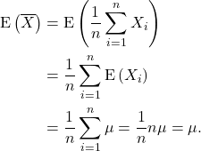
First consider the mean of ![]() . We use properties of expectation and variance of a sum of independent random variables.
. We use properties of expectation and variance of a sum of independent random variables.

Similarly,
![Rendered by QuickLaTeX.com \[{\rm Var}\left(\overline X\right) = {\rm Var}\left(\frac{1}{n}\sum_{i=1}^nX_i\right) = \frac{1}{n^2}\sum_{i=1}^n{\rm Var}\left(X_i\right) =\frac{1}{n^2}\sum_{i=1}^n \sigma^2 = \frac{1}{n^2} n\sigma^2 = \frac{\sigma^2}{n}.\]](https://oercollective.caul.edu.au/app/uploads/quicklatex/quicklatex.com-035b97203eec97854896363d60dca858_l3.png)
Note: Be careful!
- The sample mean is the average calculated from a sample, and is denoted
 . This is a random variable, because its value depends on the sample chosen, and the sampling is random. Its observed value calculated from sample data is denoted
  . This observed value depends on the sample data.
 - The population mean
 is a constant at any point it time. It may change with time, but at the time of sampling we assume it is a constant. The value of
  is usually unknown.
9.2 Sampling Distribution of the Sample Mean
- In many sampling situations the population mean
 is unavailable and is the parameter of interest.
 - The natural way to estimate
 is by the sample mean
  .
. - For inference about
 , we need the distribution of the sample mean
  .
. - The distribution of
 depends on the population distribution and the sampling scheme, and so it is called the sampling distribution of the sample mean.
 - The sampling distribution of the sample mean depends on the population variance
 .
. - Different sampling distributions arise, depending on whether
 is known or not.
 - The population distribution is often unknown.
We consider three cases below. These three cases from the basis of estimation and inference and will be used throughout the rest of the book.
Case 1: Normal population—σ known
Let ![]() be iid
be iid ![]() random variables. Then
random variables. Then
![]()
or
![]()
This follows from our earlier results that sums and linear scaling of normal random variables are also normal.
We saw this result in the simulation histograms earlier, where we had simulated from a normal distribution.
Example 9.4
The time it takes to serve a customer at a bank teller is normal with mean 150 secs and variance 900 secs![]() .
.
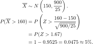
(i) What is the probability that a random sample of 25 customers will have a mean service time greater than 160 seconds?
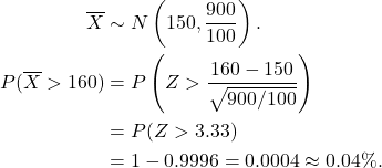
(ii) Repeat (i) above for a sample of 100 customers.
Solution
(i) Let ![]() denote the sample mean. Then
denote the sample mean. Then

(ii)Now

Example 9.5
A sample of size 100 is drawn from a N![]() population. Find
population. Find
(i) ![]()
(ii) ![]()
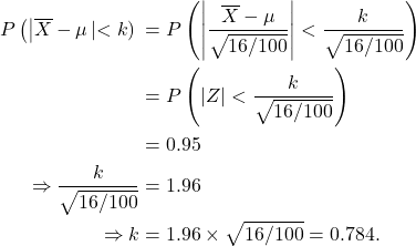
(iii) ![]() such that
such that ![]() .
.
Solution
(i) ![]() , since the normal distribution is symmetric about its mean.
, since the normal distribution is symmetric about its mean.
(ii)
![Rendered by QuickLaTeX.com \begin{align*} P\left(\left | \overline X - \mu\left | < 0.2\right) &= P\left(\left |\frac{\overline X - \mu}{\sqrt{16/100}}\right | < \frac{0.2}{\sqrt{16/100}}\right)\\ &= P(\left|Z\right| < 0.5) \\ &= 2\times [P(Z < 0.5) - 0.5]\\ &= 2\times(0.6915 - 0.5) = 0.3830. \end{align*}](https://oercollective.caul.edu.au/app/uploads/quicklatex/quicklatex.com-dfb208e659006a83539ac63cf8e2c80c_l3.png)
(iii)

Case 2: Normal Population—σ Unknown
Now we estimate the population standard deviation by the sample standard deviation ![]() . Then
. Then
![]()
where ![]() is a t distribution with
is a t distribution with ![]() degrees of freedom.
degrees of freedom.
The ![]() -distribution has a similar shape to that of the standard normal distribution, but is flatter. We say the
-distribution has a similar shape to that of the standard normal distribution, but is flatter. We say the ![]() -distribution has “fatter tails”. For large values of degrees of freedom (df), the
-distribution has “fatter tails”. For large values of degrees of freedom (df), the ![]() -distribution is very close to the normal distribution. The plot below shows the density functions for the standard normal distribution with several
-distribution is very close to the normal distribution. The plot below shows the density functions for the standard normal distribution with several ![]() -distributions superimposed.
-distributions superimposed.
Notes
-
![Rendered by QuickLaTeX.com \[S^2 = \frac{1}{n-1} \sum_{i= 1}^n \left(X_i - \overline X\right)^2\]](https://oercollective.caul.edu.au/app/uploads/quicklatex/quicklatex.com-c328d59d9ae6f199a7d370e45cbe4a04_l3.png) is the estimator of
is the estimator of  . The divisor in this expression is
  , which is the degrees of freedom of the
  -distribution. ALWAYS the divisor in the estimator for the variance gives the df for the corresponding t distribution for the problem.
 -
![Rendered by QuickLaTeX.com \[Var\left(\overline X\right) = \frac{\sigma^2}{n},\]](https://oercollective.caul.edu.au/app/uploads/quicklatex/quicklatex.com-38594e86ef888ee36512e1713690132b_l3.png)
and this is estimated by
![Rendered by QuickLaTeX.com \[\frac{S}{\sqrt{n}} = {\rm \ standard\ error\ (SE)\ of\ the\ mean.}\]](https://oercollective.caul.edu.au/app/uploads/quicklatex/quicklatex.com-aff8f2140354744792d3a0e52e862b28_l3.png)
t-tables
![]() -tables list the
-tables list the ![]() -values for only the tail probabilities of given degrees of freedom. But R give probabilities for all values for all degrees of freedom.
-values for only the tail probabilities of given degrees of freedom. But R give probabilities for all values for all degrees of freedom.
> pnorm(1.95) ##P(Z < 1.95) for Z ~ N(0,1)
[1] 0.9744119
> pt(1.95, 5) ##P(T < 1.95) for T ~ t_5 distribution
[1] 0.9456649
> pt(1.95, 20) ##P(T < 1.95) for T ~ t_20 distribution
[1] 0.9673328
> pt(1.95, 200) ##P(T < 1.95) for T ~ t_100 distribution
[1] 0.9737131
Case 3: Population Not Normal—σ Unknown
CENTRAL LIMIT THEOREM (CLT)
Suppose ![]() are iid random variables with mean
are iid random variables with mean ![]() and variance
and variance ![]() . If
. If ![]() is large enough, then
is large enough, then
![]()
Notes
- We consider
 to be large enough for the approximation to be good. As
  increases the approximation improves.
If ![]() is unknown then
is unknown then
![]()
BUT we must have ![]() .
.
Notes
- If the sample size is large (a few hundred), then the
 can be approximated by N
 distribution. This is the most common situation.
 - Although historically the N(0,1) distribution has been used in hand calculations, R ALWAYS uses the
 distribution.
Example 9.6
A particular long-life light bulb has a mean life of 1500 hours with a standard deviation of 300 hours. What is the probability that a random sample of 200 bulbs has a mean life time less than 1450 hours?
Solution
Here the standardised sample mean is
![]()
by the CLT (![]() ).
).

9.3 Summary
| Population standard deviation |
Normal distribution | Not normal distribution |
|---|---|---|
| Known |
Exact distribution |
Approximate distribution |
| Unknown |
Exact distribution |
Approximate distribution |

