3 Probability
Learning Outcomes
At the end of this chapter you should be able to:
- use the axioms of probability to prove simple probability results;
- use the axioms of probability to solve problems involving probabilities;
- understand the concept of conditional probability and use it to solve problems;
- know the multiplication rule and use it to solve problems;
- understand the concepts of independence and disjoint (mutually exclusive)
events, and use these to solve problems; - solve probability problems using tree diagrams.
Brief history of Probability
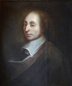
A gambler’s dispute in 1654 led to the creation of a mathematical theory of probability by two French mathematicians, Blaise Pascal and Pierre de Fermat. Antoine Gombaud (who called himself Chevalier de Méré, meaning Knight of Mé’ré), a French noble man and a writer with an interest in gaming and gambling questions, called Pascal’s attention to an apparent contradiction concerning a popular dice game.
Reproduced under a CC BY 3.0 licence from WikiMedia Commons.
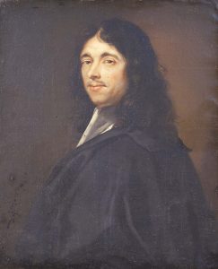
Copy of oil on canvas painting by Roland Lefevre. Public Domain artwork sourced from WikiMedia Commons
The problem
The game consisted of throwing a pair of dice 24 times. The problem was to decide whether or not to bet even money on the occurrence of at least one double six during the 24 throws. A seemingly well-established gambling rule led de Méré to believe that betting on a double six in 24 throws would be profitable. But his own calculations showed just the opposite.
This problem posed by de Méré and others led to an exchange of letters between Pascal and Fermat in which the fundamental principles of probability were formulated for the first time.
Question: What is the probability of winning in the above game if you bet on “at least one double six”?
Contents
3.1 Notation and terminology
A random phenomenon is one for which the outcome cannot be predicted with certainty in advance. A random experiment is a process that generates outcomes that can only be described in terms of probabilities. Examples of common random events are tossing a coin and rolling a die.
Sample space
A sample space, denoted  , is the set of all possible outcomes of a random experiment. Any outcome in the sample space is called an elementary event. An event is a subset of the sample space.
Example 3.1
If a coin is tossed twice then the sample space is  Then
Then  is an elementary event. Further,
  is an event, which can be described in words as at least one H.
Assigning probabilities
The probability of an event  is the number of outcomes in the sample space favourable to divided by the total number of outcomes, that is
![\[{\rm P}(A) = \frac{\# \ {\rm of\ outcomes\ favourable\ to\ } A}{\rm Total\ number\ of\ outcomes}.\]](https://oercollective.caul.edu.au/app/uploads/quicklatex/quicklatex.com-7d7e7218b0ae2b095947389095da1236_l3.png "Rendered by QuickLaTeX.com")
Note that this assignment assumes that the outcomes are equally likely.
Example 3.1 (ctd)
If we toss a coin twice, then

The null or empty event
The null event or empty event is denoted  (phi) and contains no outcomes.
Example 3.1 (ctd)
Toss a coin twice. The event “Obtaining 3 H” is a null event–we cannot get three H from two tosses of a coin.
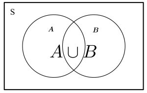
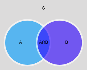
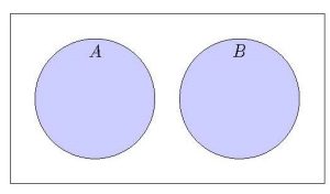
Union and Intersection
The union of and  is denoted
  , and is the set of points that are in or or both. The intersection of two sets and is denoted
  , and is the set of points that are in both and . We often say or to indicate union, and and to indicate intersection. These relationships can be represented by Venn diagrams, as below.
Complementary and Disjoint Events
is denoted  or
or  , and is the set of points that are not in . This is illustrated in the Venn diagram below. and are mutually exclusive or disjoint if
  , that is, and have no intersection. Disjoint events have no points in common.
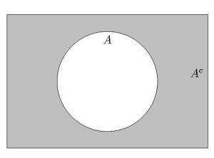
- What is the complement of ?
- What is the intersection of and ?
Note that  , the entire sample space.
Example 3.2
Two coins are tossed. Let denote the event that the first toss yields a H.
(a) What is the complement of ?
(b) Specify some events that are disjoint with .
Solution
(a) Here
![\[S = \{HH, HT, TH, TT\}, A = \{HH, HT\}, A^c = \{TH, TT\}.\]](https://oercollective.caul.edu.au/app/uploads/quicklatex/quicklatex.com-b34bee62ec893a84a31e6cc962ddd39c_l3.png "Rendered by QuickLaTeX.com")
(B) is disjoint with .  and
and  are also disjoint with .
3.2 Axioms of probability
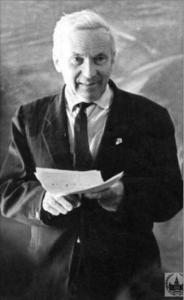
Reproduced under a CC BY-SA 4.0 DEED license from WikiMedia Commons
Kolmogorov (1903-1987), a Soviet mathematician, one of the most influential mathematicians of the twentieth century, put probability on a firm mathematical foundation (1933). He also contributed to topology, intuitionistic logic, turbulence, classical mechanics, algorithmic information theory and computational complexity.
He postulated the following three axioms of probability.
A1.  . (Something must happen.)
A2.  for any event .
A3. If and are disjoint then
![\[P(A\cup B) = P(A) + P(B).\]](https://oercollective.caul.edu.au/app/uploads/quicklatex/quicklatex.com-c2416b970386b02cb0252ba1119ce56b_l3.png "Rendered by QuickLaTeX.com")
Exercise
Draw a Venn diagram to represent Axiom A3.
3.3 Rules of Probability
Based on the axioms of probability we can derive the following rules. For any events and ,
P1. 
P2. 
P3. 
P4. 
Proof
P1. .
Note that and are disjoint since  . Also,
  and , so

P2. .
and are disjoint, since  . Also, . Then

Note that it also follows that  .
.
P3. .
By A2 , or  . Also by A2,
  . But
. But
![\[P(A) = 1-\underbrace{P(A^c)}_{\ge 0} \le 1.\]](https://oercollective.caul.edu.au/app/uploads/quicklatex/quicklatex.com-49e6a3320c64bb041ade0f36797d4329_l3.png "Rendered by QuickLaTeX.com")
It follows that .
P4.  .
.
Note that  and
and  are disjoint sets, and
  ). Then by A3,
![\[P(A) = P(A\cap B) + P(A \cap B^c) \Rightarrow P(A\cap B^c) = P(A) - P(A\cap B).\]](https://oercollective.caul.edu.au/app/uploads/quicklatex/quicklatex.com-fff5056bdb93c083e2c889a14bcfa1dd_l3.png "Rendered by QuickLaTeX.com")
Further, and  are disjoint sets, and
Now

Note that  is sometimes read as “P(A) equals probability of with plus probability of without “. This is a form of the Theorem of total probabilities. The event
  is also read as only occurs.
Example 3.3
Let  and
and  . Calculate
(a) P(at least one of and occurs)
(b) P(only occurs)
(c) P(neither nor occurs)
Solution
(a) 
(b) The event “only occurs” is represented by . Now

(c) Neither nor occurs is equivalent to  , so
, so
![\[P[(A\cup B)^c] = 1- P(A\cup B) = 1- 0.6 = 0.4.\]](https://oercollective.caul.edu.au/app/uploads/quicklatex/quicklatex.com-4358e3f8ad97f2a950455d8106747f65_l3.png "Rendered by QuickLaTeX.com")
A Venn diagram can be used to illustrate this situation.
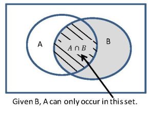
3.4 Conditional Probability
For events and , the probability of occurring when it is known that has occurred is called the conditional probability of given , denoted
![\[P(A|B),\]](https://oercollective.caul.edu.au/app/uploads/quicklatex/quicklatex.com-73a348831c0cf2af79aca90134da094f_l3.png "Rendered by QuickLaTeX.com")
read as “probability of given “. Note that  is a probability, so it satisfies ALL the axioms and rules for probabilities.
Definition
If and are two events such that  , then
![\[P(A|B) = \frac{P(A \cap B)}{P(B)}.\]](https://oercollective.caul.edu.au/app/uploads/quicklatex/quicklatex.com-8465e55b9c6f0a30be0c254e430071c4_l3.png "Rendered by QuickLaTeX.com")
Since has occurred, the sample space is now only , and the probability that occurs is the proportion of where occurs. This is illustrated in the Venn diagram below.
Example 3.4 Bank data
The table below lists the number of bank workers by gender and job-grade.
| Job Grade | |||||||
|---|---|---|---|---|---|---|---|
| 1 | 2 | 3 | 4 | 5 | 6 | Total | |
| Female | 48 | 29 | 36 | 17 | 9 | 1 | 140 |
| Male | 12 | 13 | 7 | 11 | 12 | 13 | 68 |
| Total | 60 | 42 | 43 | 28 | 21 | 14 | 208 |
Data source ©Cengage Learning Inc. Reproduced by permission. www.cengage.com/permissions
Using the information in the table, calculate the following probabilities.
(a) An employee selected at random at job grade higher than 4 is a male.
(b) A female employee selected at random is at a job grade higher than 4.
(c) An employee selected at random at job grade below 5 is a female.
Solution
(a) We are given the employee is at Job Grade higher than 4, so we need
![\[P(Male|Job\ Grade \ge 5) = \frac{25}{35} = \frac{5}{7} \approx 0.7143.\]](https://oercollective.caul.edu.au/app/uploads/quicklatex/quicklatex.com-f323cdc165526303b9ef38a703140459_l3.png "Rendered by QuickLaTeX.com")
(b) Here we know the employee is female, so the required probability is
![\[P(Job\ Grade \ge 5|Female) = \frac{10}{140} = \frac{1}{14} \approx 0.0714.\]](https://oercollective.caul.edu.au/app/uploads/quicklatex/quicklatex.com-52d7ef269a1555f158be179d3ae120ca_l3.png "Rendered by QuickLaTeX.com")
(c) Now we know the employee is at Job Grade below 5, so
![\[P(Female|Job\ Grade \le 4) =\frac{130}{173} \approx 0.7514.\]](https://oercollective.caul.edu.au/app/uploads/quicklatex/quicklatex.com-1a52459ec2dcf787e57e692b392f742b_l3.png "Rendered by QuickLaTeX.com")
Proportionally more females are at lower Job Grades.
3.5 Multiplication Rules
The conditional probability rule is
![\[P(A|B) = \frac{P(A\cap B)}{P(B)},\]](https://oercollective.caul.edu.au/app/uploads/quicklatex/quicklatex.com-d45da7e2ab3e2a90804a9367d1bf0b58_l3.png "Rendered by QuickLaTeX.com")
from which we obtain
![\[P(A\cap B) = P(B) \times P(A|B).\]](https://oercollective.caul.edu.au/app/uploads/quicklatex/quicklatex.com-f27bdb382739b020fdcf6682b4b82a6b_l3.png "Rendered by QuickLaTeX.com")
Similarly from
![\[P(B|A) = \frac{P(A\cap B)}{P(A)}\]](https://oercollective.caul.edu.au/app/uploads/quicklatex/quicklatex.com-0bf39d608c30b614758d22e075c9c904_l3.png "Rendered by QuickLaTeX.com")
we obtain
![\[P(A\cap B) = P(A) \times P(B|A).\]](https://oercollective.caul.edu.au/app/uploads/quicklatex/quicklatex.com-9a793d2963efe7f9770f80ea97fe040e_l3.png "Rendered by QuickLaTeX.com")
That is, we can obtain  as
as
![\[PA\cap B) = P(A) \times P(B|A) = P(B) \times P(A|B).\]](https://oercollective.caul.edu.au/app/uploads/quicklatex/quicklatex.com-76b7e45f39c0fd94207fead9ff0c227f_l3.png "Rendered by QuickLaTeX.com")
This rule essentially says that for and to occur together,
- first occurs, and then occurs given has occurred, OR
- first occurs and then occurs given has occurred.
3.6 Tree Diagrams
Tree diagrams can be used to facilitate the solution of conditional probability problems. They implement the multiplication rule and the rule of total probabilities. This is illustrate in the tree diagram below.
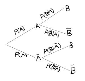
To calculate the probability for any event we simply multiply the probabilities along the path of the event. For example, the path for is along the top branches of the tree, so this probability is found by multiplying the probabilities of the branches, that is,
Similarly,
![\[P(\overline A\cap B) = P(\overline A) \times P(B|\overline A).\]](https://oercollective.caul.edu.au/app/uploads/quicklatex/quicklatex.com-798dae710ba015c0929c55e92fbf0cca_l3.png "Rendered by QuickLaTeX.com")
Note that the probabilities along branches that originate at the same node sum to 1.
The use of tree diagrams to solve probability problems is illustrated in the following example.
Example 3.5
Machines and turn out respectively 10% and 90% of the total production of a certain type of article. The probability Machine produces a defective article is 0.01, while that for Machine is 0.05. A randomly selected article from a day’s production is defective. What is the probability the article was made by Machine A?
Solution
The solution to these probability problems can be quite tricky. We outline the steps that one needs to follow to solve such problems efficiently and simply.
Step 1. Define appropriate events. Let denote the event that an item is produced by Machine and  denote the event that the item is defective.
Note that it might seem as if there are four events: an item is produced by Machines or , and an item is defective or not. But the other two events (item is produced by Machine , item is defective) are the complements of the defined events.
Step 2. Express given probabilities in terms of these events and draw a tree diagram to represent this information.
![\[P(A) = 0.1, P(B) = 0.9, P(D|A) = 0.01, P(D|\overline A) = 0.05.\]](https://oercollective.caul.edu.au/app/uploads/quicklatex/quicklatex.com-091cfb5364a6c0363681e82f2505d637_l3.png "Rendered by QuickLaTeX.com")
Note that it follows that  and
and  . The tree diagram is given below.

Step 3. Express the required probability in terms of the defined events, and calculate it using the probability rules and the tree diagram.
We need  . Sometimes identifying the required probability is difficult. In the problem statement above we have highlighted the probability statement, which indicates that we need the probability of the event , that is, the article was made by machine A, and the rest of the information is the given or conditional part of the probability statement. Using the conditional probability rule we get
(1) 
Note that one could go from the first line straight to the third line, following the path along the two branches in which the event occurs.
Example 3.6
Consider again the data of Example 3.4.
| Job Grade |
|||||||
|---|---|---|---|---|---|---|---|
| 1 | 2 | 3 | 4 | 5 | 6 | Total | |
| Female | 48 | 29 | 36 | 17 | 9 | 1 | 140 |
| Male | 12 | 13 | 7 | 11 | 12 | 13 | 68 |
| Total | 60 | 42 | 43 | 28 | 21 | 14 | 208 |
Data source ©Cengage Learning Inc. Reproduced by permission. www.cengage.com/permissions
What is the probability that an employee picked at random
(a) is female and is at Job Grade 5 or above?
(b) at Job Grade 4 or below is male?
(c) at Job Grade 5 or above is female?
(d) at Job Grade 5 or above is male?
On the basis of the above calculations, what can be concluded about the promotion culture in the bank?
Solution
Let the event  denote the employee is male and the event
  that Job Grade is 5 or above.
(a) 
(b) 
(c) 
(d) 
The probability of being at a higher Job Grade for females is less than 30%, indicating that there is a gender bias in promotions. BUT, this does not adjust for differences in education, experience, and other variables that may affect promotion.
3.7 Independent events
Intuitively, two events and are independent if the occurrence of one does not affect the probability of the occurrence of the other. Formally, events and are independent if
(2) 
Otherwise the two events are dependent.
Notes
- To determine if two events are independent, the above condition in equation (2) needs to be verified.
- If and are independent events than
![\[P(A|B) = \frac{P(A \cap B)}{P(B)} = \frac{P(A) \times P(B)}{P(B)} = P(A)},\]](https://oercollective.caul.edu.au/app/uploads/quicklatex/quicklatex.com-53e6771bb40d12edb9fe0c6bc75c491e_l3.png "Rendered by QuickLaTeX.com")
so the occurrence of
does not affect the probability of occurrence of . - Similarly,
![\[P(B|A) = \frac{P(A \cap B)}{P(A)} = \frac{P(A) \times P(B)}{P(A)} = P(B)},\]](https://oercollective.caul.edu.au/app/uploads/quicklatex/quicklatex.com-8f7860d7ce43f6d229d9f4182a5ecf6a_l3.png "Rendered by QuickLaTeX.com")
so the occurrence of
does not affect probability of the occurrence of .
This is intuitively what independence means. That is, if two events are independent than the occurrence of one does not affect the probability of the occurrence of the other.
Do not confuse mutually exclusive and independence.
Events and are mutually exclusive (or disjoint) if
![\[P(A \cap B) = 0.\]](https://oercollective.caul.edu.au/app/uploads/quicklatex/quicklatex.com-d43921caada82d1745b3cac61e565777_l3.png "Rendered by QuickLaTeX.com")
Events and are independent if
![\[P(A\cap B) = P(A) \times P(B).\]](https://oercollective.caul.edu.au/app/uploads/quicklatex/quicklatex.com-3c4a2f76252839f9385bbfc19747ddc1_l3.png "Rendered by QuickLaTeX.com")
Example 3.7 Bank Data
Consider again the data of Example 3.4.
| Job Grade |
|||||||
|---|---|---|---|---|---|---|---|
| 1 | 2 | 3 | 4 | 5 | 6 | Total | |
| Female | 48 | 29 | 36 | 17 | 9 | 1 | 140 |
| Male | 12 | 13 | 7 | 11 | 12 | 13 | 68 |
| Total | 60 | 42 | 43 | 28 | 21 | 14 | 208 |
Data source ©Cengage Learning Inc. Reproduced by permission. www.cengage.com/permissions
(a) Let denote the event that an employee is male, and be the event that the employee is at Job Grade 5 or above. Are the events and independent?
(b) Is gender independent of Job Grade? If not, what is the relationship between gender and Job Grade?
Solution
(a) From the table,
![\[P(M) = \frac{68}{208}, P(J) = \frac{35}{208}, P(M \cap J) = \frac{25}{208} \approx 0.1208.\]](https://oercollective.caul.edu.au/app/uploads/quicklatex/quicklatex.com-3eca74c039005ce55d32ca21a103603f_l3.png "Rendered by QuickLaTeX.com")
Then
![\[P(M) \times P(J) = \frac{68}{208} \times \frac{35}{208} \approx 0.0551 \ne P(M\cap J).\]](https://oercollective.caul.edu.au/app/uploads/quicklatex/quicklatex.com-89c6a10d08e8828fc6f71e4cf82ebd9e_l3.png "Rendered by QuickLaTeX.com")
Thus and are NOT independent.
(b) Gender and Job Grade are dependent by part (a) above. Males are more likely to be at higher Job Grades and females are more likely to be at lower Job Grades.
Example 3.8
A woman is selling her house. She believes that there is a 0.3 chance that a person who inspects her house will purchase it. Assuming that the people inspecting the house decide independently whether or not to purchase the house, what is the probability that more than two people will inspect the house before it is sold?
Solution
Let  denote the event that the first person to view the house buys it, and let
  denote the event that the second person to view the house buys it. Then and are independent. If more than two people view the house before it is sold, then this means that the first two to view the house do not buy it. This is represented by the event
  . Since and are independent, so are
  and
and  (see result below). Then
![\[P(\overline A_1 \cap \overline A_2) = P(\overline A_1) \times P(\overline A_2) = (1-0.3) \times (1-0.3) = 0.49.\]](https://oercollective.caul.edu.au/app/uploads/quicklatex/quicklatex.com-289a2f0e7ef08ddfcdc92c9a0915f5d0_l3.png "Rendered by QuickLaTeX.com")
Result
If events and are independent, then the pairs of events  and , and
  , and are also independent.
Exercise Prove this result.
3.8 Exercise
Draw a tree diagram for Example 4.8.
Example 3.9
While searching for oil in Australia, an oil explorer orders seismic tests to determine if oil is likely to be found in a certain drilling area. The following probabilities summarise past results concerning the reliability of the test: when oil does exist in the testing area, the test will indicate so 85% of the time; when oil does not exist in the testing area, the probability is 0.03 that the test will erroneously indicate that oil does exist. Preliminary exploration by geologists indicates that the probability of the existence of oil deposits in the test area is 0.45. If the seismic test is conducted and indicates the presence of oil, what is the probability that an oil deposit really does exist?
Solution
Let  denote the event that oil is present and
  denotes the event that the test indicates the presence of oil. Then
  . The tree diagram below represents this information.

We need

