10 Estimation
Learning Outcomes
At the end of this chapter you should be able to:
- explain the difference between point and interval estimates;
- understand the concept of a confidence interval;
- compute a confidence interval for a population mean;
- compute the confidence interval for a population proportion;
- explain the factors that affect the width of a confidence interval;
- interpret confidence intervals;
- compute the required sample size for a given error.
Contents
10.1 Introduction
Population parameters are usually unknown. What is the mean age of Australians? What is the median house price in Perth suburbs? How much do international students need for living expenses?
We use an appropriate sample statistic, ![]() , to estimates a population parameter
, to estimates a population parameter ![]() . We call
. We call ![]() the estimator of
the estimator of ![]() . The observed value of
. The observed value of ![]() , denoted
, denoted ![]() , is an estimate of
, is an estimate of ![]() . For example,
. For example, ![]() is an estimator of population mean
is an estimator of population mean ![]() , and
, and ![]() is an estimate of
is an estimate of ![]() .
.
![]() is an unbiased estimator of parameter
is an unbiased estimator of parameter ![]() if
if ![]() .
.
10.2 Common Estimators
We are interested mainly in estimating population mean ![]() and population proportion
and population proportion ![]() .
.
Population Mean 
The sample mean
![]()
is an unbiased estimator of the population mean ![]() .
.
![]()
Population Variance 
The sample variance
![]()
is an unbiased estimator of the population variance ![]() .
.
Proof
To prove that the sample variance is an unbiased estimator of the population variance we need to show that the expected value of the sample variance is equal to the population variance. First note that from properties of variance,
![]()
This gives the following two results, with ![]() replaced by
replaced by ![]() and
and ![]() as appropriate.
as appropriate.
![Rendered by QuickLaTeX.com \begin{align*} {\rm E}(X_i^2) &= {\rm Var}(X_i) + \left[{\rm E}(X_i)\right]^2 = \sigma^2 + \mu^2,\\ {\rm E}({\overline X}^2) &= {\rm Var}(\overline X) + \left[{\rm E}(\overline X)\right]^2 = \frac{\sigma^2}{n} + \mu^2. \end{align*}](https://oercollective.caul.edu.au/app/uploads/quicklatex/quicklatex.com-28753894e53e14c61c5c56e617e73329_l3.png)
Next, note that from properties of sums from chapter 3,
![]()
Then
![Rendered by QuickLaTeX.com \begin{align*} {\rm E}\left[(n-1)S^2\right] &= {\rm E}\left[\sum_{i=1}^n \left(X_i-\overline X\right)^2\right]= {\rm E}\left[\sum_{i=1}^n X_i^2 - n{\overline X}^2\right]\\ &= \sum_{i=1}^n {\rm E}\left(X_i^2\right) -n{\rm E}\left({\overline X}^2 \right)\\ &= \sum_{i=1}^n \left(\sigma^2 + \mu^2\right) - n \left(\frac{\sigma^2}{n} + \mu^2\right)\\ &= n\ \sigma^2 + n\ \mu^2 - \sigma^2 - n\ \mu^2= (n-1)\sigma^2,\\ \intertext{so} {\rm E}\left(S^2\right) &= \sigma^2. \end{align*}](https://oercollective.caul.edu.au/app/uploads/quicklatex/quicklatex.com-d42bb682451e4809108583233bb74511_l3.png)
That is, the sample variance is an unbiased estimator for the population variance.
Population Proportion 
The sample here is ![]() identical Bern(
identical Bern(![]() ) trials (e.g. toss a coin
) trials (e.g. toss a coin ![]() times). Let
times). Let ![]() denote the outcome of the trials, so
denote the outcome of the trials, so
![]()
Then the sample proportion
![]()
is an unbiased estimator of the population proportion, where
![]()
Proof
Note that ![]() are iid and
are iid and ![]() . Put
. Put
![]()
so ![]() is the number of successes in
is the number of successes in ![]() iid Bernoulli trials. Thus
iid Bernoulli trials. Thus ![]() , so
, so
![]()
Now put
![]()
Note that ![]() denotes the sample proportion of successes. Then
denotes the sample proportion of successes. Then
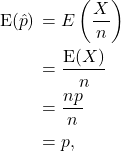
so ![]() is an unbiased estimator for the population proportion
is an unbiased estimator for the population proportion ![]() . Further,
. Further,
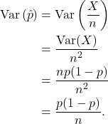
In practice ![]() is unknown, so we estimate
is unknown, so we estimate ![]() by
by ![]() . Then the standard error of
. Then the standard error of ![]() is
is
![]()
Distribution of 
Note that
![]()
where ![]() are iid Bern
are iid Bern![]() random variables. So
random variables. So ![]() is simply a sample mean. Then all the results of Chapter 10 apply. In particular, for
is simply a sample mean. Then all the results of Chapter 10 apply. In particular, for ![]() , by CLT,
, by CLT,
![]()

10.3 Confidence Intervals
A point estimate does not include any measure of variability. An interval estimate is often preferred, as it also includes a measure of the variability of the estimate.
10.3.1 Confidence interval for population mean µ
![]() is a point estimate of
is a point estimate of ![]() . We choose a confidence level, say 95%. We need two symmetric limits,
. We choose a confidence level, say 95%. We need two symmetric limits, ![]() and
and ![]() , such that
, such that
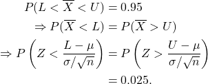
Now for the normal distribution, ![]() , so we have
, so we have

Then
![]()
We want end points that are not based on ![]() . Thus
. Thus
![]()
Similarly,
![]()
This gives
![]()
and
![]()
From this we obtain a 95% confidence interval (CI) for ![]() as
as
![]()
Note that this is a random interval (since ![]() is a random variable). In practice, we use the estimate
is a random variable). In practice, we use the estimate ![]() for
for ![]() , giving an observed 95% CI for
, giving an observed 95% CI for ![]() as
as
![]()
In general, a ![]() CI is given by
CI is given by
![]()
where ![]()
or
![]()
The appropriate ![]() can be obtained using software.
can be obtained using software.
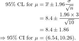
Example 10.1 Compute a 95% confidence interval for a population mean ![]() based on sample of size
based on sample of size ![]() , with
, with ![]() .
.
Solution
The confidence limits (CL) are
Frequentist interpretation of confidence interval
We still do not know the value of ![]() . Thus we do not know if any given (observed) CI contains
. Thus we do not know if any given (observed) CI contains ![]() or not. We cannot say in Example 10.1 that
or not. We cannot say in Example 10.1 that
![]()
However, if several samples of size ![]() are taken and a 95% CI computed for each, then 95% of these intervals will on average contain the value of
are taken and a 95% CI computed for each, then 95% of these intervals will on average contain the value of ![]() . This is illustrated in the figure below. Twenty random samples of size 100 each were taken from a N
. This is illustrated in the figure below. Twenty random samples of size 100 each were taken from a N![]() distribution. The 95% confidence intervals obtained from these samples are given in the figure below, with the horizontal line representing the population mean
distribution. The 95% confidence intervals obtained from these samples are given in the figure below, with the horizontal line representing the population mean ![]() . Of these, only one (that is, 5%) does not contain the value of the sample mean.
. Of these, only one (that is, 5%) does not contain the value of the sample mean.
Accuracy of estimate
The half-width of the interval is ![]() This depends on three things.
This depends on three things.
- Level of confidence. High confidence
 larger value of
  wider interval.
 - The standard deviation
 . Large
  wide interval. Large
  indicates large variance in the population, and hence larger uncertainty in the estimate.
 - Sample size
 . Large sample size
  narrow interval.
Of these three parameters, only the sample size can be controlled. A narrow (more accurate) interval with high confidence requires a larger sample size, which comes at a cost.
Sampling distribution again
In Chapter 10 we covered three cases for the distribution of the sample mean. These three cases apply in the calculation of the confidence interval.
CASE 1 Normal Population — ![]() known (RARELY THE CASE)}
known (RARELY THE CASE)}
![]() CL =
CL = ![]()
CASE 2 Normal Population — ![]() unknown
unknown
![]() CL =
CL = ![]()
CASE 3 Population Distribution not Normal
Use CLT ![]() .
.
![]() CL =
CL = ![]()
OR if ![]() is large (a few hundred) use
is large (a few hundred) use ![]() .
.
If ![]() then we must assume that the population is normal and use Case 2 (since
then we must assume that the population is normal and use Case 2 (since ![]() is usually unknown).
is usually unknown).
Note R always uses the t-distribution. Historically the normal distribution is used for hand calculations for ease, since table values for all degrees of freedom for the t-distribution are not available.
General form of confidence interval
General form of ![]() CL for parameter
CL for parameter ![]() is
is
![]()
OR
![]()
Example 10.2
Chronic exposure to asbestos fibre is a well known health hazard. The table below gives measurements of pulmonary compliance (a measure of the how effectively the lung can inhale and exhale, in ml/ cm H![]() O) for 16 construction workers, 8 months after they had left a site on which they had suffered prolonged exposure to asbestos. (Data source: Harless, Watanabe and Renzetti Jr (1978). `The Acute Effects of Chrysotile Asbestos Exposure on Lung Function’, Environmental Research, 16, 360-372. ©Elsevier. Used with permission.)
O) for 16 construction workers, 8 months after they had left a site on which they had suffered prolonged exposure to asbestos. (Data source: Harless, Watanabe and Renzetti Jr (1978). `The Acute Effects of Chrysotile Asbestos Exposure on Lung Function’, Environmental Research, 16, 360-372. ©Elsevier. Used with permission.)
Table: Pulmonary compliance (ml/ cm H![]() O) for 16 workers subjected to prolonged exposure to asbestos fibre.
O) for 16 workers subjected to prolonged exposure to asbestos fibre.
| 167.9 | 180.8 | 184.8 | 189.8 | 194.8 | 200.2 | 201.9 | 206.9 |
| 207.2 | 208.4 | 226.3 | 227.7 | 228.5 | 232.4 | 239.8 | 258.6 |
Compute a point estimate and a 95% confidence interval for the population mean pulmonary compliance ![]() for people with prolonged asbestos fibre exposure.
for people with prolonged asbestos fibre exposure.
Solution
The mean of the data is ![]() and the sample standard deviation is
and the sample standard deviation is ![]() . The standard error for
. The standard error for ![]() is
is ![]() . To find a 95% confidence interval for
. To find a 95% confidence interval for ![]() , we need the critical value
, we need the critical value ![]() with
with ![]() , where
, where ![]() (since 95% = 100(1-0.05)). From R we find that
(since 95% = 100(1-0.05)). From R we find that ![]() . Hence, a 95% confidence interval for
. Hence, a 95% confidence interval for ![]() is given by
is given by

Example 10.3
A random sample of 200 light bulbs gives a mean lifetime of 2,000 hours with a standard deviation of 150 hours. Find a 95% confidence interval for the mean lifetime ![]() of the bulbs.
of the bulbs.
Solution
![]() and
and ![]() . The value of
. The value of ![]() from R is 1.972. Note the value is negative, since we obtained the lower 0.025 critical value.
from R is 1.972. Note the value is negative, since we obtained the lower 0.025 critical value.
qt(0.025,199)
[1] -1.971957
Then

so 95% CI ![]() hours.
hours.
Example 10.4
To estimate the mean weekly income of restaurant waitresses in a large city, an investigator collects weekly income data from a random sample of 75 waitresses. The mean and standard deviation are found to be $200 and $30 respectively. Compute a 99% confidence interval for the mean weekly income.
Solution
![]() and
and ![]() . The value of
. The value of ![]() from R is 2.6439. Note that the value is negative, since we obtained the lower 0.005 critical value.
from R is 2.6439. Note that the value is negative, since we obtained the lower 0.005 critical value.
qt(0.005,74)
[1] -2.643913
Then

so 99% CI ![]() ($190.84, $209.16).
($190.84, $209.16).
10.3.2 Confidence Interval for Population Proportion
We consider only the case ![]() . Then the standardised sample proportion is
. Then the standardised sample proportion is
![Rendered by QuickLaTeX.com \[Z=\dfrac{\hat{p}-p}{\sqrt{\dfrac{p(1-p)}{n}}} \sim \textrm{N(0,1)}.\]](https://oercollective.caul.edu.au/app/uploads/quicklatex/quicklatex.com-931e8050481a9f8f0d2b65fbd16bb614_l3.png)
Note that ![]() , Var
, Var![]() . Since
. Since ![]() is unknown, we estimate it by
is unknown, we estimate it by ![]() , and estimate
, and estimate

![]()
The half-width of the interval is ![]() ,
,
and depends on three things.
- Level of confidence. High confidence
 wider interval.
  . Close to 0.5
  wider interval, close to 0 or 1
  narrow interval.
 . Large
 narrow interval.
Example 10.5
A random sample of 100 children in a developing country found that 15% of them were classified as low birth weight (< 2500 g). Compute a 95% CI for the population proportion of babies that are low birth weight (LBW).
Solution
The sample proportion of LBW babies is ![]() . Then
. Then

10.4 Sample size calculations
Here we assume that the sample size is large (at least ![]() , but usually a few hundred) so we can use the normal distribution (instead of the
, but usually a few hundred) so we can use the normal distribution (instead of the ![]() -distribution). The error in estimating a parameter by an interval estimate is half the interval width.
-distribution). The error in estimating a parameter by an interval estimate is half the interval width.
Population Mean
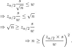
The half width is ![]() . If we want this to be less than
. If we want this to be less than ![]() , then
, then
Example 10.6
What minimum sample size is required to estimate a population mean to within ![]() with 95% confidence if
with 95% confidence if ![]() ?
?
Solution
Assume ![]() so we can use the normal distribution. Then
so we can use the normal distribution. Then
![]()
that is, ![]() .
.
In practice we would take ![]() as a round figure.
as a round figure.
Population proportion
The half width is ![]() where
where ![]() is the standard deviation of the Bern
is the standard deviation of the Bern![]() observations that comprise the sample.
observations that comprise the sample.
So the formula for the sample size is the same is previously:
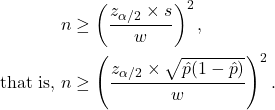
This depends on the value of ![]() , which is unknown before the sample is taken! However, the expression
, which is unknown before the sample is taken! However, the expression ![]() is greatest when
is greatest when ![]() . Thus we can take:
. Thus we can take:
![]()
Example 10.7
What minimum sample size is required to estimate a population proportion to within 0.05 with confidence 95%?
Solution
Assume ![]() so we can use the normal distribution. Then
so we can use the normal distribution. Then
![]()
that is, ![]() .
.
In practice we would take ![]() as a round figure.
as a round figure.
10.5 Summary
Population mean
![]()
Population proportion
![]()

