6.5 Null Hypothesis Testing
In the first chapter, we discussed the three major goals of statistics: to describe, decide and predict. So far, we have talked about how we can use statistics to describe. In the next few sections, we will introduce the ideas behind the use of statistics to make decisions – in particular, decisions about whether a particular hypothesis is supported by the data.
The specific type of hypothesis testing that we will discuss is known (for reasons that will become clear) as null hypothesis statistical testing (NHST). You would be very familiar with this concept if you ever read any scientific literature. In their introductory psychology textbook, Gerrig et al. (2002)[1] referred to NHST as the “backbone of psychological research”. Thus, learning how to use and interpret the results from hypothesis testing is essential to understanding the results from many fields of research.
It is also important for you to know, however, that NHST is deeply flawed, and that many statisticians and researchers (including myself) think that it has been the cause of serious problems in science. For more than 50 years, there have been calls to abandon NHST in favour of other approaches (like those that we will discuss in the following chapters).
NHST is also widely misunderstood, largely because it violates our intuitions about how statistical hypothesis testing should work. Let’s look at an example to see this.
Null Hypothesis Statistical Testing
There is great interest in the use of body-worn cameras by police officers, which are thought to reduce the use of force and improve officer behaviour. However, to establish this we need experimental evidence, and it has become increasingly common for governments to use randomised controlled trials to test such ideas. A six-month randomized controlled trial of the effectiveness of body-worn cameras was performed by Western Australia Police Force in 2016.[2] Throughout the trial, days were assigned randomly as either “treatment” days, where all participating officers began their shifts wearing and using body-worn cameras, or “control” days, when no officers used body-worn cameras. The study measured four different outcomes, impact on: 1) cost and time efficiencies during field interviews, 2) rates of guilty pleas, 3) sanction rates and police use of force, and 4) citizen’s complaints against police and assaults against police.
Before we get to the results, let’s ask how you would think the statistical analysis might work. Let’s say we want to specifically test the hypothesis of whether police use of force is decreased by the wearing of cameras. The randomised controlled trial provides us with the data to test the hypothesis – namely, the rates of use of force by officers on the day they were assigned to either the camera or control (i.e., no camera). The next obvious step is to look at the data and determine whether they provide convincing evidence for or against this hypothesis. That is: What is the likelihood that body-worn cameras reduce the use of force, given the data and everything else we know?
It turns out that this is not how null hypothesis testing works. Instead, we first take our hypothesis of interest (i.e. that body-worn cameras reduce the use of force), and flip it on its head, creating a null hypothesis – in this case, the null hypothesis would be that cameras do not reduce use of force. Importantly, we then assume that the null hypothesis is true. We then look at the data, and determine how likely the data would be if the null hypothesis were true.
If there is insufficient evidence to reject the null, then we say that we retain (or “fail to reject”) the null, sticking with our initial assumption that the null is true. If, however, there is sufficient evidence to say that the null hypothesis is not true – then we can we reject the null in favour of the alternative hypothesis (which is our hypothesis of interest).
If your head was boggled after reading the sentences above, don’t worry, you won’t be the only one.
Understanding some of the concepts of NHST, particularly the notorious “p-value”, is invariably challenging the first time one encounters them, because they are so counter-intuitive. As we will see later, there are other approaches that provide a much more intuitive way to address hypothesis testing (but have their own complexities). However, before we get to those, it’s important for you to have a deep understanding of how hypothesis testing works, because it’s clearly not going to go away any time soon.
Null-Hypothesis Statistical Testing – An Intuitive Explanation
As mentioned above, the idea behind the NHST is so counter-intuitive. However, this is an important concept to understand as it is not going away anytime soon. The most intuitive explanation for NHST is applying it to the courtroom.
Imagine you’re in a courtroom, and you’re on trial for a crime. In this analogy, you are the defendant, and the legal system has its own way of approaching the case, somewhat like null hypothesis testing in statistics. In court, you start with the presumption of innocence. This is similar to the “null hypothesis” in statistics. The null hypothesis assumes that there is no real difference or effect; it’s like saying, “innocent until proven guilty.” The opposite of the null hypothesis is the “alternative hypothesis.” In our trial analogy, this would mean suspected of being guilty. It’s the opposite of innocence.
In court, both the prosecution and defence present evidence to support their arguments. Similarly, in null hypothesis testing, you collect data and analyse it to see if there’s enough evidence to reject the null hypothesis in favour of the alternative hypothesis. In court, the burden of proof is on the prosecution. They need to provide enough evidence to convince the jury (or judge) that the person being convicted is guilty. Similarly, in statistics, the burden of proof is on the data. We need to collect enough evidence to decide whether the null hypothesis is unlikely to be true.
In court, if there is not enough evidence to prove guilt (beyond a reasonable doubt), the defendant is declared innocent. Similarly, in NHST, if the data doesn’t provide enough evidence to reject the null hypothesis, we retain it.
The Process of Null Hypothesis Testing
We can break the process of null hypothesis testing down into a number of steps:
-
Formulate a hypothesis – we should formulate a hypothesis that embodies our prediction (before seeing the data)
- Specify null and alternative hypotheses
- Collect some data relevant to the hypothesis
- Fit a model to the data that represents the alternative hypothesis and compute a test statistic
- Compute the probability of the observed value of that statistic assuming that the null hypothesis is true
- Assess the “statistical significance” of the result.
For a hands-on example, let’s use the NHANES data to ask the following question: Is physical activity related to body mass index? In the NHANES dataset, participants were asked whether they engage regularly in moderate or vigorous-intensity sports, fitness or recreational activities (variable named PhysActive). The researchers also measured height and weight and used them to compute the Body Mass Index (BMI).
Step 1: Formulate a Hypothesis
We hypothesise that BMI is greater for people who do not engage in physical activity, compared to those who do.
Step 2: Specify the Null and Alternative Hypotheses
For step 2, we need to specify our null hypothesis (which we call H0) and our alternative hypothesis (which we call HA – we also sometimes see it as H1, H2 and so on). H0 is the baseline against which we test our hypothesis of interest: that is, what would we expect the data to look like if there was no effect? The null hypothesis always involves some kind of equality (e.g., ==, equals to)
HA describes what we expect if there actually is an effect. The alternative hypothesis always involves some kind of inequality (≠≠, >, or <, not equal to, greater than or less than). Importantly, null hypothesis testing operates under the assumption that the null hypothesis is true unless the evidence shows otherwise.
We also have to decide whether we want to test a directional or non-directional hypotheses. A non-directional hypothesis simply predicts that there will be a difference, without predicting which direction it will go. For the BMI/activity example, a non-directional null hypothesis would be:

In words: There is no difference in BMI between people who do not engage in physical activity compared to those who do.

In words: There will be a difference in BMI between people who do not engage in physical activity compared to those who do.
A directional hypothesis, on the other hand, predicts which direction the difference would go. For example, we have strong prior knowledge to predict that people who engage in physical activity should weigh less than those who do not, so we would propose the following directional alternative hypothesis:

As we will see later, testing a non-directional hypothesis is more conservative, so this is generally preferred unless there is a strong a priori reason to hypothesise an effect in a particular direction. Hypotheses, including whether they are directional or not, should always be specified prior to looking at the data!
Step 3: Collect Some Data
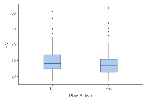
In this case, we will sample around 5% of the adults (age 18 and over) from the NHANES dataset. Figure 6.5.1 shows an example of such a sample, with BMI shown separately for active and inactive individuals, and Table 6.5.1. shows summary statistics for each group.
Table 6.5.1. Summary of BMI data for active versus inactive individuals
| Descriptives | |||||||||||
|---|---|---|---|---|---|---|---|---|---|---|---|
| PhysActive | N | Missing | Mean | SD | |||||||
| BMI | No | 137 | 3 | 29.67 | 7.50 | ||||||
| Yes | 152 | 1 | 27.65 | 6.80 | |||||||
Step 4: Fit a Model to the Data and Compute a Test Statistic
Next, we want to use the data to compute a statistic that will ultimately let us decide whether the null hypothesis is rejected or not. To do this, the model needs to quantify the amount of evidence in favour of the alternative hypothesis, relative to the variability in the data. Thus, we can think of the test statistic as providing a measure of the size of the effect (i.e., impact of physical activity on BMI) compared to the variability in the data (i.e., people BMI variation). In other words, we need to determine the signal from the noise (if this exists!).
In general, test statistics will have a probability distribution associated with it, because that allows us to determine how likely our observed value of the statistic is under the null hypothesis. If this doesn’t make sense, hopefully, the intuitive explanation below will clear this up.
For the BMI example, we need a test statistic that allows us to test for a difference between two means, since the hypotheses are stated in terms of mean BMI for each group. One statistic that is often used to compare two means is the t statistic, first developed by the statistician William Sealy Gossett, who worked for the Guinness Brewery in Dublin and wrote under the pen name “Student” – hence, it is often called “Student’s t statistic”. The t statistic is appropriate for comparing the means of two groups when the sample sizes are relatively small and the population standard deviation is unknown.
Those truly interested in looking at the formula can see it at the end of this chapter, but essentially, the t statistic is a way of quantifying how large the difference between groups is in relation to the sampling variability. In our case, this is the difference between those who are physically active and those who are not LARGE enough compared to the BMI variability you would find in the sample. If the groups that we have are roughly the same size and have equal variance, then we can go ahead and calculate our t statistic and the the degrees of freedom for the t test is the number of observations minus 2 (N – 2). In our example, we should have the degrees of freedom of 287 (289 – 2).
However, it can be seen from the box plot that the inactive group is more variable than the active group and that there are more people who are active (n = 152) compared to those who are inactive (n = 137). Therefore, we need to use a corrected calculation for our degrees of freedom, which is often referred to as a “Welch t test”. Using the corrected test, we should get the degrees of freedom of 275.83, which is slightly smaller than the degrees of freedom calculated above. This in effect imposes a “penalty” on the test for differences in sample size or variance.
Step 5: Determine the Probability of the Observed Result Under the Null Hypothesis
Determining the probability of the observed result under the null hypothesis is a fundamental aspect of hypothesis testing. It’s like asking, “How likely is it that what we’ve seen is just due to random chance?” This is also where it breaks our intuition.
Read the excerpt below as I try to explain the concepts behind probability and null hypothesis as intuitively as I can.
Is your $1 coin fair? Intuition behind probability and null hypothesis
Imagine that you had an inkling that $1 coins are biased – you think that it may be tails-heavy, meaning that $1 coins are more likely to land heads up. In this scenario, the null hypothesis is that it’s a fair coin. If $1 coins are fair, then the coin will have a 50% chance of landing heads up and a 50% chance of landing tails up. Therefore,
- H0 = coin is fair
- HA = coin is head-biased
Let’s say you got a bunch of $1 coins to flip and flipped them 100 times and we plot the frequency of getting a particular number of landing on tails on a graph and its probability of getting that result (see Figure 6.5.2).
In your coin toss, you got 52 heads. Does that give you some doubts that maybe the coin is not fair after all? Well, maybe not because the probability of getting 52 heads out of 100 flips is still quite high (see below). In fact, if we use a probability calculator, the probability of getting at least 52 heads is 0.38 or 38% chance of success. 38% is quite close to 50% – so it could be just by chance that we got 52 heads out of 100 tosses.
What if, in our 100 tosses, we got 66 heads instead? Maybe doubts are starting to form. Around 2 thirds of the tosses are coming up as heads. If you can see that the 66 heads out of 100 tosses got you questioning the fairness of the coin (compared to the other sample) – then congratulations, you have the right mindset to understand the intuition behind hypothesis testing!
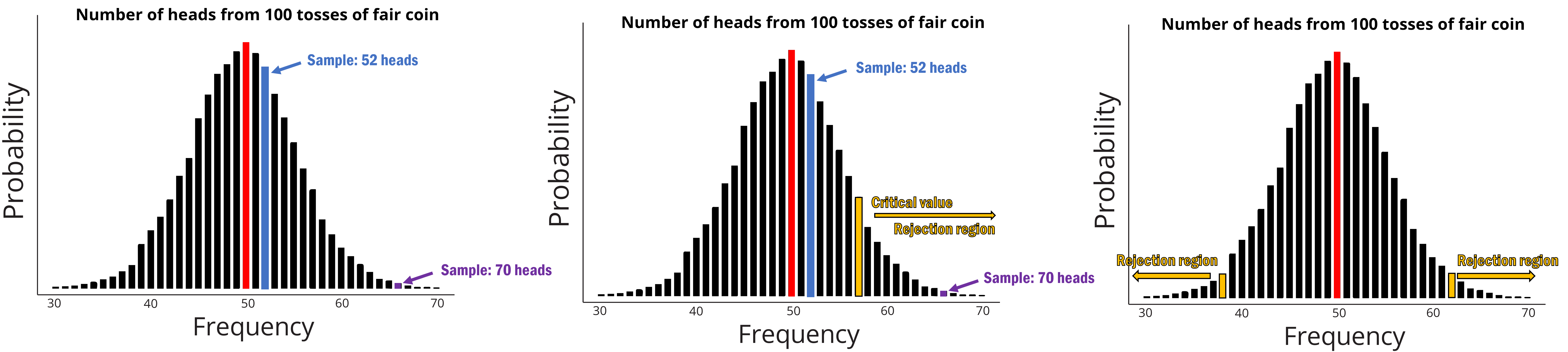
Basically, when we conduct NHST, we are essentially testing if the result that we get is extreme enough. We then make a decision that this result is not due to chance. With the example we provided above, the probability of getting at least 66 heads is 0.00089 – in other words, there is only 0.089% chance that we will get 66 heads out of 100 tosses!
As researchers, we try to make it easy on ourselves by appointing a value that we use to decide whether our result is rare enough to reject the null hypothesis. This is where critical values come in. Critical values are designated points in which we are happy to say that the result is rare enough that it may not be due to chance. Critical values can either be on only one side of the probability distribution (Figure 6.5.2 – middle panel) or on both sides of the probability distribution (Figure 6.5.2 – left panel).
Our hypothesis determines whether we use one side or two sides of the probability distribution (we call these one-tailed or two-tailed tests). If we are asking if the coin is biased in general (i.e., we don’t know whether it is tail-biased or head-biased) then you will use these two critical points. If our results fall beyond either side of the critical value region, then we can reject the null hypothesis. If we are asking if the coin is only head-biased (or tail-biased) then we will use the one-tailed test. If our results fall beyond on our chosen side of the critical value region, then we can reject the null hypothesis.
Computing p-Values Using the t Distribution
Now, let’s go back to our BMI example and compute a p-value for our BMI example using the t distribution. First, we compute the t statistic using the values from our sample that we calculated above, where we find that t = 2.38. The question that we then want to ask is: What is the likelihood that we would find a t statistic of this size, if the true difference between groups is zero (i.e. the directional null hypothesis)?
We can use the t distribution to determine this probability. According to jamovi, the probability value (or more commonly known as p-value) of getting t = 2.38 with a df of 275.83 is 0.018. In other words, our p-value is 0.018. This tells us that our observed t statistic value of 2.38 is relatively unlikely if the null hypothesis really is true.
The p-value provided in jamovi is usually set to non-directional hypothesis as a default (see under Hypothesis, the Group 1 =\= Group 2 will be selected). If we want to use a directional hypothesis (in which we only look at one end of the null distribution), then we click the option Group 1 > Group 2 or Group 1 < Group 2. What you choose will depend on what you have written for your hypothesis.
In our data, group 1 was the physically non-active group and group 2 is the physically active group. If we used the one-tailed test with Group 1 > Group 2, then we get a p-value of 0.009. Here, we see that the p value for the two-tailed test is twice as large as that for the one-tailed test, which reflects the fact that an extreme value is less surprising since it could have occurred in either direction.
How do you choose whether to use a one-tailed versus a two-tailed test?
The two-tailed test is always going to be more conservative, so it’s always a good bet to use that one unless you had a very strong prior reason for using a one-tailed test. In that case, you should have written down the hypothesis before you ever looked at the data. In Chapter 4, we discussed the idea of pre-registration of hypotheses, which formalises the idea of writing down your hypotheses before you ever see the actual data. You should never make a decision about how to perform a hypothesis test once you have looked at the data, as this can introduce serious bias into the results.
Step 6: Assess the “Statistical Significance” of the Result
The next step is to determine whether the p-value that results from the previous step is small enough that we are willing to reject the null hypothesis and conclude instead that the alternative is true. How much evidence do we require? This is one of the most controversial questions in statistics, in part because it requires a subjective judgment – there is no “correct” answer.
Historically, the most common answer to this question has been that we should reject the null hypothesis if the p-value is less than 0.05. This comes from the writings of Ronald Fisher, who has been referred to as “the single most important figure in 20th-century statistics” (Efron 1998):
If P is between .1 and .9 there is certainly no reason to suspect the hypothesis tested. If it is below .02 it is strongly indicated that the hypothesis fails to account for the whole of the facts. We shall not often be astray if we draw a conventional line at .05 … it is convenient to draw the line at about the level at which we can say: Either there is something in the treatment, or a coincidence has occurred such as does not occur more than once in twenty trials. (Fisher, 1925)[3]
However, Fisher never intended p < 0.05 to be a fixed rule:
no scientific worker has a fixed level of significance at which from year to year, and in all circumstances, he rejects hypotheses; he rather gives his mind to each particular case in the light of his evidence and his ideas. (Fisher, 1956)[4]
Instead, it is likely that p < 0.05 became a ritual due to its simplicity – before computing, people had to rely on reading tables of p-values. Since all tables had an entry for 0.05, it was easy to determine whether one’s statistic exceeded the value needed to reach that level of significance.
The choice of statistical thresholds remains deeply controversial, and researchers have been proposing to change the default threshold to be more conservative (e.g., 0.05 to 0.005), making it substantially more stringent and thus more difficult to reject the null hypothesis. In large part, this move is due to growing concerns that the evidence obtained from a significant result at p < 0.05 is relatively weak.
Hypothesis Testing as Decision-Making: The Neyman-Pearson Approach
Whereas Fisher thought that the p-value could provide evidence regarding a specific hypothesis, the statisticians Jerzy Neyman and Egon Pearson disagreed vehemently. Instead, they proposed that we think of hypothesis testing in terms of its error rate in the long run:
no test based upon a theory of probability can by itself provide any valuable evidence of the truth or falsehood of a hypothesis. But we may look at the purpose of tests from another viewpoint. Without hoping to know whether each separate hypothesis is true or false, we may search for rules to govern our behaviour with regard to them, in following which we insure that, in the long run of experience, we shall not often be wrong. (Neyman & Pearson 1933)[5]
That is: We can’t know which specific decisions are right or wrong, but if we follow the rules, we can at least know how often our decisions will be wrong in the long run.
To understand the decision making framework that Neyman and Pearson developed, we first need to discuss statistical decision making in terms of the kinds of outcomes that can occur. There are two possible states of reality (H0 is true or H0 is false) and two possible decisions (reject H0 or retain H0).
There are two ways in which we can make a correct decision:
- We can reject H0 when it is false (in the language of signal detection theory, we call this a hit).
- We can retain H0 when it is true (somewhat confusingly in this context, this is called a correct rejection).
There are also two kinds of errors we can make:
- We can reject H0 when it is actually true (we call this a false alarm, or Type I error).
- We can retain H0 when it is actually false (we call this a miss, or Type II error).
Neyman and Pearson coined two terms to describe the probability of these two types of errors in the long run:
- P(Type I error) =
- P(Type II error) =
That is, if we set to 0.05, then in the long run we should make a Type I error 5% of the time. Whereas it’s common to set as 0.05, the standard value for an acceptable level of is 0.2 – that is, we are willing to accept that 20% of the time we will fail to detect a true effect when it truly exists. We will return to this later when we discuss statistical power, which is the complement of Type II error.
What does a Significant Result Mean?
There is a great deal of confusion about what p-values actually mean (Gigerenzer, 2004).[6] Let’s say that we do an experiment comparing the means between conditions, and we find a difference with a p-value of .05. There are a number of possible interpretations that one might entertain.
Does it mean that the probability of the null hypothesis being true is 0.01?
No. Remember that in null hypothesis testing, the p-value is the probability of the data given the null hypothesis. For those who think in formula, p-value is calculated as P(data|H0). It does not warrant conclusions about the probability of the null hypothesis given the data – this suggestsP(H0|data).
Does it mean that the probability that you are making the wrong decision is 0.01?
No – this suggests P(H0|data). But remember as above that p-values are probabilities of data under H0 – not the other way around.
Does it mean that if you ran the study again, you would obtain the same result 99% of the time?
No. The p-value is a statement about the likelihood of a particular dataset under the null; it does not allow us to make inferences about the likelihood of future events such as replication.
Does it mean that you have found a practically important effect?
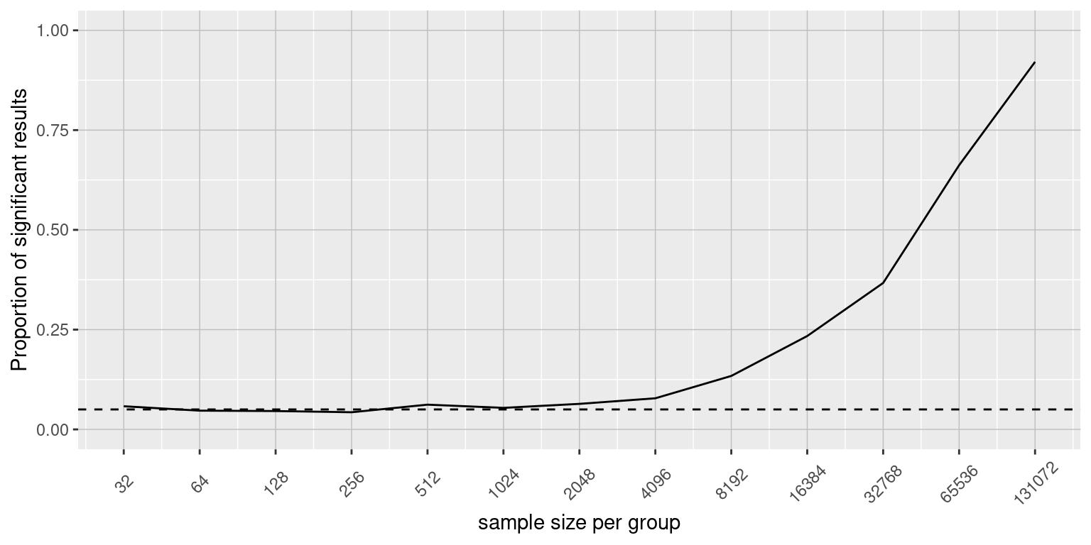
No. There is an essential distinction between statistical significance and practical significance. As an example, let’s say that we performed a randomised controlled trial to examine the effect of a particular diet on body weight, and we find a statistically significant effect at p<.05. What this doesn’t tell us is how much weight was actually lost, which we refer to as the effect size (to be discussed in more detail later on. If we think about a study of weight loss, then we probably don’t think that the loss of one ounce (i.e. the weight of a few potato chips) is practically significant. Let’s look at our ability to detect a significant difference of 1 ounce as the sample size increases.
Figure 6.5.3 shows how the proportion of significant results increases as the sample size increases, such that with a very large sample size (about 262,000 total subjects), we will find a significant result in more than 90% of studies when there is a 1 ounce difference in weight loss between the diets. While these are statistically significant, most physicians would not consider a weight loss of one ounce to be practically or clinically significant. We will explore this relationship in more detail when we return to the concept of statistical power in the next few section, but it should already be clear from this example that statistical significance is not necessarily indicative of practical significance.
In summary, being able to reject the null hypothesis is indirect evidence of the experimental or alternative hypothesis. However, rejecting the null hypothesis
- DOES NOT say whether the scientific conclusion is correct.
- DOES NOT tell us anything about the mechanism behind any differences or the relationship (e.g., does not tell us WHY there’s a difference in BMI compared with physically active and physically inactive adults).
- DOES NOT tell us whether the study is well designed or well controlled.
- DOES NOT PROVE ANYTHING.
Chapter attribution
This chapter contains material taken and adapted from Statistical thinking for the 21st Century by Russell A. Poldrack, used under a CC BY-NC 4.0 licence.
Screenshots from the jamovi program. The jamovi project (V 2.2.5) is used under the AGPL3 licence.
- Gerrig, R. J., Zimbardo, P. G., Campbell, A. J., Cumming, S. R., & Wilkes, F. J. (2015). Psychology and life. Pearson Higher Education. ↵
- Clare, J., Henstock, D., McComb, C., Newland, R., & Barnes, G. C. (2021). The results of a randomized controlled trial of police body-worn video in Australia. Journal of Experimental Criminology, 17(1), 43–54. https://link.springer.com/article/10.1007/s11292-019-09387-w ↵
- Fisher, R. A. 1925. Statistical methods for research workers. Oliver & Boyd. ↵
- Efron, B. (1998). R. A. Fisher in the 21st Century (invited paper presented at the 1996 R. A. Fisher Lecture). Statistical Science, 13(2), 95–122. https://doi.org/10.1214/ss/1028905930. ↵
- Neyman, J., and K. Pearson. 1933. On the problem of the most efficient tests of statistical hypotheses. Philosophical Transactions of the Royal Society of London A: Mathematical, Physical and Engineering Sciences 231(694-706): 289–337. https://doi.org/10.1098/rsta.1933.0009. ↵
- Gigerenzer, G. (2004). Fast and frugal heuristics: The tools of bounded rationality. In D. J. Koehler & N. Harvey (Eds.), Blackwell handbook of judgment and decision making (pp. 62–88). Blackwell Publishing. https://doi.org/10.1002/9780470752937.ch4 ↵
