Anyone living in Australia will be familiar with the concept of sampling from the political polls that have become a central part of our electoral process. In some cases, these polls can be incredibly accurate at predicting the outcomes of elections.

Nate Silver, an American statistician, was named one of the globe’s top 100 influential individuals by Time magazine in 2009 after correctly predicting electoral outcomes for 49/50 states in 2008 (he had a better outcome in 2012 when he correctly predicted all 50 states). Silver did this by combining data from 21 different polls, which vary in the degree to which they tend to lean towards either the Republican or Democratic side. Each of these polls included data from about 1000 likely voters – meaning that Silver was able to almost perfectly predict the pattern of votes of more than 125 million voters using data from only about 21,000 people, along with other knowledge (such as how those states have voted in the past).

We don’t have an equivalent of Nate Silver in Australia, but a recent article by the Australian Financial Review stated that Australian polls are getting more reliable.^[1] According to the AFR, pollsters attribute the uptick in accuracy to better sampling methods. 

How do we Sample?

Our goal in sampling is to determine the value of a statistic for an entire population of interest, using just a small subset of the population. We do this primarily to save time and effort – why go to the trouble of measuring every individual in the population when just a small sample is sufficient to accurately estimate the statistic of interest?

In the election example, the population is all registered voters in the region being polled, and the sample is the set of 1000 individuals selected by the polling organisation. The way in which we select the sample is critical to ensuring that the sample is representative of the entire population, which is the main goal of statistical sampling. It’s easy to imagine a non-representative sample; if a pollster only called individuals whose names they had received from the local Greens Party, then it would be unlikely that the results of the poll would be representative of the population as a whole. In general, we would define a representative poll as being one in which every member of the population has an equal chance of being selected. When this fails, then we have to worry about whether the statistic that we computed using the sample is biased – that is, whether its value is systematically different from the population value (which we will refer to as a parameter). Keep in mind that we generally don’t know this population parameter, because if we did then we wouldn’t need to sample!

However, every now and again, we will use examples that have access to entire populations in order to explain some key ideas about sampling. Like the example used below.

Sampling Error and Standard Error of the Mean

Regardless of how representative our sample is, it’s likely that the statistic that we compute from the sample is going to differ at least slightly from the population parameter. We refer to this as sampling error.

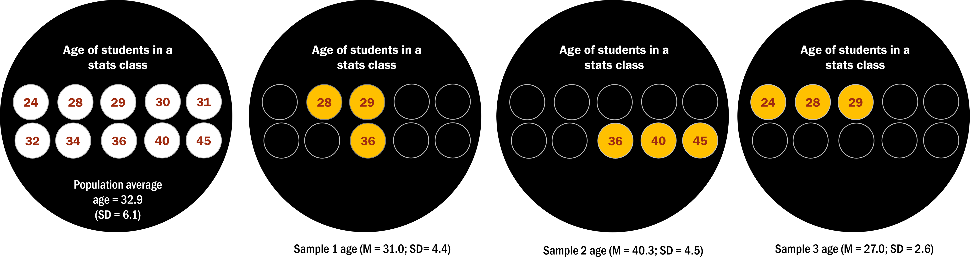
Suppose I wanted to know the average age of students in my stats class. The population average is 32.9 – this is the number that I am interested in knowing.  However, it is usually rare to know the population parameter. In our example, maybe some of the students in the class are not comfortable sharing their age. So, instead, we take a sample.

Let’s say we ask three people in the class and the responses we receive are 28, 29, and 36 years. By calculating the average of these ages, we obtain a sample mean of 31.0. This number is not too different from the population mean of 32.9. However, what if we get sample 2’s average instead (see Figure 6.3.1 below), consisting of individuals aged 36, 40, and 45. In this sample, we have a mean of 40.3 – this sample has a larger sampling error. Yet again, we conducted another sampling, where the ages reported were 24, 28, and 29, and calculated the average age for this new group, we would obtain a sample of 27.0.

The amount of variation between the average age of the different samples is a measure of sampling error. Sampling error is directly related to the quality of our measurement of the population. Clearly we want the estimates obtained from our sample to be as close as possible to the true value of the population parameter. However, even if our statistic is unbiased (that is, we expect it to have the same value as the population parameter), the value for any particular estimate will differ from the population value, and those differences will be greater when the sampling error is greater. Thus, reducing sampling error is an important step towards better measurement.

As you can see, it’s important to characterise how variable our sample is, in order to make inferences about the sample statistic. If sampling error is the difference between a sample statistic and its corresponding population parameter, then the standard error of the mean (SEM) is a measure of how much sampling error is expected in the sample mean. In other words, the SEM is telling you how much discrepancy you can expect between the sample mean and the true population mean.

To compute SEM, we divide the estimated standard deviation by the square root of the sample size:

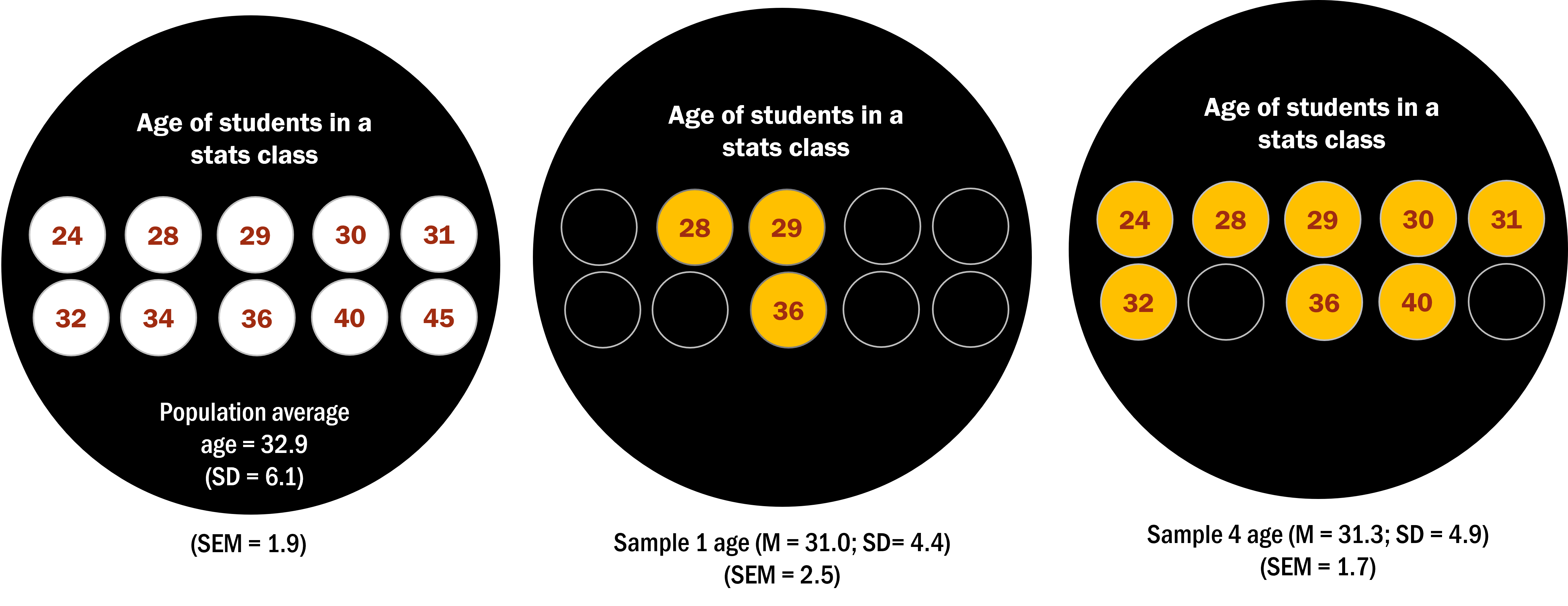
with s as the standard deviation of the sample, and n is the sample size. Looking at the formula, you can intuitively see that the quality of our estimate will be dependent on two things, the variability of the population and the size of the sample. In other words, the larger the sample we have, the more accurate it will be in estimating the population mean due to a lower SEM. As you can see in Figure 6.3.2, the SEM for sample 4 with an n of 8 is much closer to the population SEM, compared to sample 1 with an n of 3.

If the variation in the population is large, then we should expect a more noisy estimate. We have no control over the population variability, but we do have control over the sample size. Thus, if we wish to improve our sample statistics (by reducing their sampling variability) then we should use larger samples. However, the formula also tells us something very fundamental about statistical sampling – namely, that the utility of larger samples diminishes with the square root of the sample size. This means that doubling the sample size will not double the quality of the statistics; rather, it will improve it by a factor of . Later on, we will discuss statistical power, which is intimately tied to this idea.