5.4 The Middle of the Data
Creating tables or drawing pictures of the data as seen previously is an excellent way to convey the gist of what the data is trying to tell you. It’s often extremely useful to try to condense the data into a few simple summary statistics. In most situations, the first thing that you’ll want to calculate is a measure of central tendency. That is, you’d like to know something about where the “average” or “middle” of your data lies. The three most commonly used measures are the mean, median and mode. I’ll explain each of these in turn, and then discuss when each of them is useful.
The Mean
Table 5.4.1 Ages of those with Crash ID 19891001, 19891002, 19891003 and 19891004
| Crash ID | Age |
| 19891001 | 66 |
| 19891002 | 42 |
| 19891003 | 18 |
| 19891004 | 76 |
The mean of these observations is:
![]()
Calculating averages in jamovi
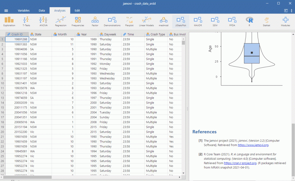
Averages (that is, means) are used so often in everyday life that this should be pretty familiar to you. We can find the average age of all people in the ARDD dataset by going to Analyses > Exploration. Drag Age into the Variables window. Under Descriptives, choose Variables across rows (this is optional – I prefer this setting because I think it looks cleaner this way). See below for the steps:

The Median
The second measure of central tendency that people use a lot is the median, and it’s even easier to describe than the mean. The median is the “middle” value. As before, let’s imagine we are only interested in the four sets of Crash ID’s we have identified earlier. To figure out the median age, we sort age into ascending order:
Table 5.4.2 Ages of those with Crash ID 19891001, 19891002, 19891003 and 19891004, highlighting the middle of the data.
| Crash ID | Age |
| 19891003 | 18 |
| 19891002 | 42 |
| 19891001 | 66 |
| 19891004 | 76 |
In this case, we will have two data in the middle, 42 and 66. If we find two data in the middle, we take the average of these two data to get the median ![]() If we only wanted to find the median of Crash ID 19891001, 19891002 and 19891003 then the middle of the dataset would be 42.
If we only wanted to find the median of Crash ID 19891001, 19891002 and 19891003 then the middle of the dataset would be 42.
Again, we do not need to do any of this by hand and we can let jamovi do the heavy lifting for us. We can find the median age in our dataset by following the same example we did above.
Mean or Median?
The mean and the median are two helpful measures. However, we need to know when we use which one. Let’s say that five people are in a bar, and we examine each person’s income (Table 5.4.3).
Table 5.4.3 Income for our five bar patrons
| income | person |
| 48000 | Bella |
| 64000 | Isaac |
| 58000 | William |
| 72000 | Gabby |
| 66000 | Alex |
The mean (61600.00) seems to be a pretty good summary of the income of those five people. Now let’s look at what happens if Beyoncé Knowles walks into the bar (Table 5.4.4).
Table 5.4.4 Income for our five bar patrons plus Beyoncé Knowles.
| income | person |
| 48000 | Bella |
| 64000 | Isaac |
| 58000 | William |
| 72000 | Gabby |
| 66000 | Alex |
| 54000000 | Beyoncé |
The mean is now almost 10 million dollars, which is not really representative of any of the people in the bar – in particular, it is heavily driven by the outlying value of Beyoncé. In general, the mean is highly sensitive to extreme values, which is why it’s always important to ensure that there are no extreme values when using the mean to summarise data.
We will go back to these concepts in the later chapters.
Mode
Calculating the mode is very simple. It is the value that occurs most frequently. Sometimes we wish to describe the central tendency of a dataset that is not numeric. For example, let’s say that we want to know which models of iPhone are most commonly used. To test this, we could ask a large group of iPhone users which model each person owns. If we were to take the average of these values, we might see that the mean iPhone model is 9.51, which is clearly nonsensical, since the iPhone model numbers are not meant to be quantitative measurements. In this case, a more appropriate measure of central tendency is the mode, the most common value in the dataset.
Similar to mean and the median, jamovi can calculate the mode by following the steps detailed above.
Chapter attribution
This chapter contains material taken and adapted from Statistical thinking for the 21st Century by Russell A. Poldrack, used under a CC BY-NC 4.0 licence.
Screenshots from the jamovi program. The jamovi project (V 2.2.5) is used under the AGPL3 licence.

