7.3 Comparing Means
Comparing a Mean to a Target Value
A straightforward question we could ask is whether a specific mean is higher or lower than a target value. For example, let’s consider testing if the average diastolic blood pressure in adults from the NHANES dataset is greater than 80, a threshold for hypertension set by the American College of Cardiology. Imagine we randomly selected 250 adults from the dataset to explore this.
We can answer this question using Student’s t-test, which you have already encountered earlier in the book. We will refer to the mean as  and the hypothesised population mean as
  . The t-test for a single mean is:

where SEM (as you may remember from the chapter on sampling) can be calculated by using the following formula:  .
.
In essence, the t =-statistic asks how large the deviation of the sample mean from the hypothesised quantity is with respect to the sampling variability of the mean.
To conduct one sample’s t-test in jamovi, go to Analyses > Exploration > but BPDiaAve into the dependent variables. Set the test value at 80. As you learned from the previous chapters, we also want jamovi to give us effect size and descriptives.
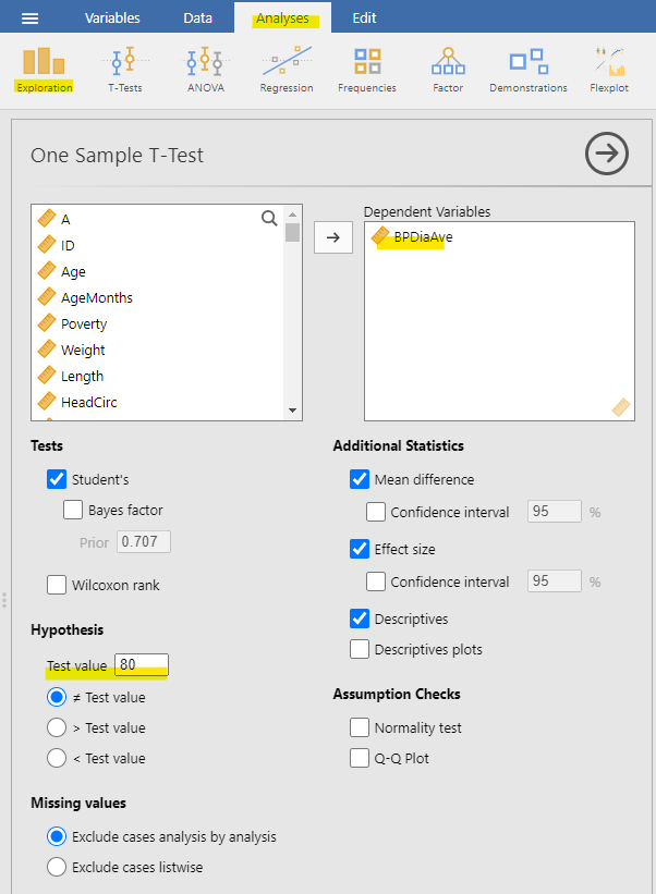
This information reveals that the mean diastolic blood pressure in the dataset (70) is significantly lower than 80. Our test to check if it’s above 80 is not even close to being statistically significant. It’s important to remember that a large p-value doesn’t offer evidence in support of the null hypothesis because we initially assumed the null hypothesis to be true.
Comparing Two Means
A more common statistical question often revolves around whether there’s a difference between the averages of two different groups. For example, let’s say we want to find out if regular marijuana smokers consume more alcohol during the day than non-regular smokers. We have the following hypothesis – smoking marijuana is linked to increased alcohol consumption (HA).
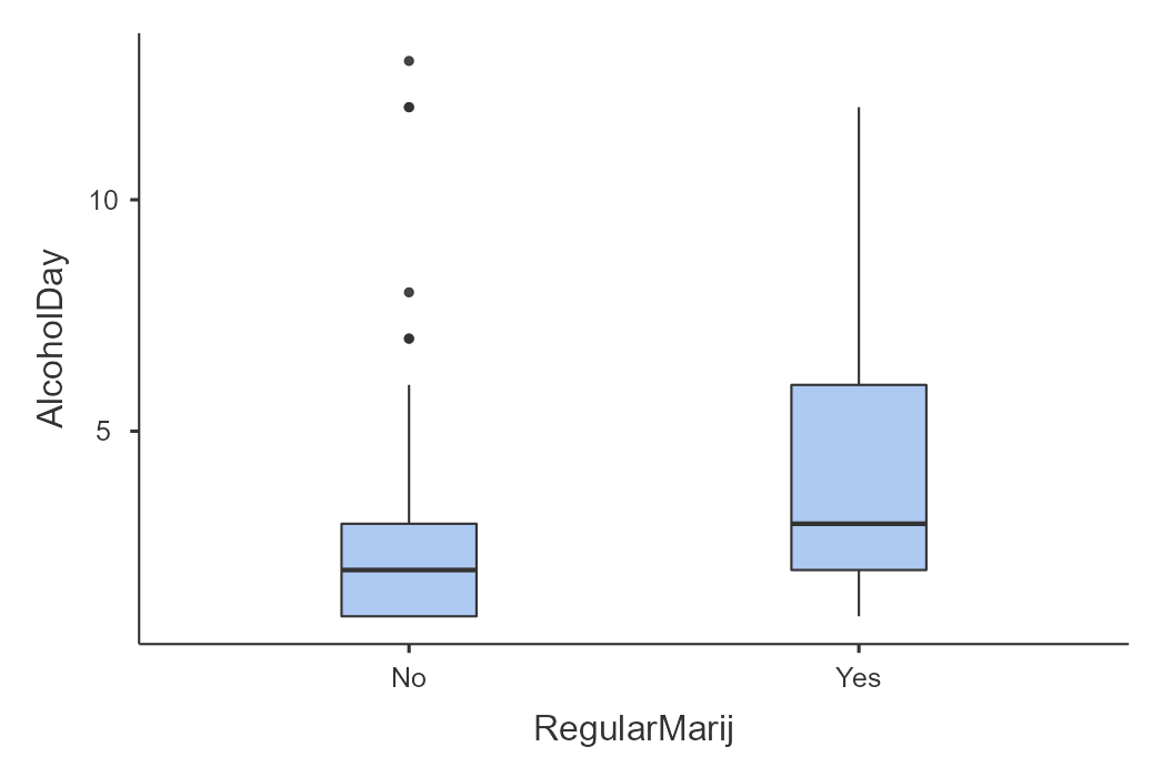
We can explore this question using the NHANES dataset. We take a sample of 5% from the dataset and investigate if the amount of alcohol consumed per year is linked to regular marijuana use. In Figure 7.3.2, you can see these data visually presented with a box plot. It’s evident that those who regularly use marijuana are also more likely to consume alcohol during the day.
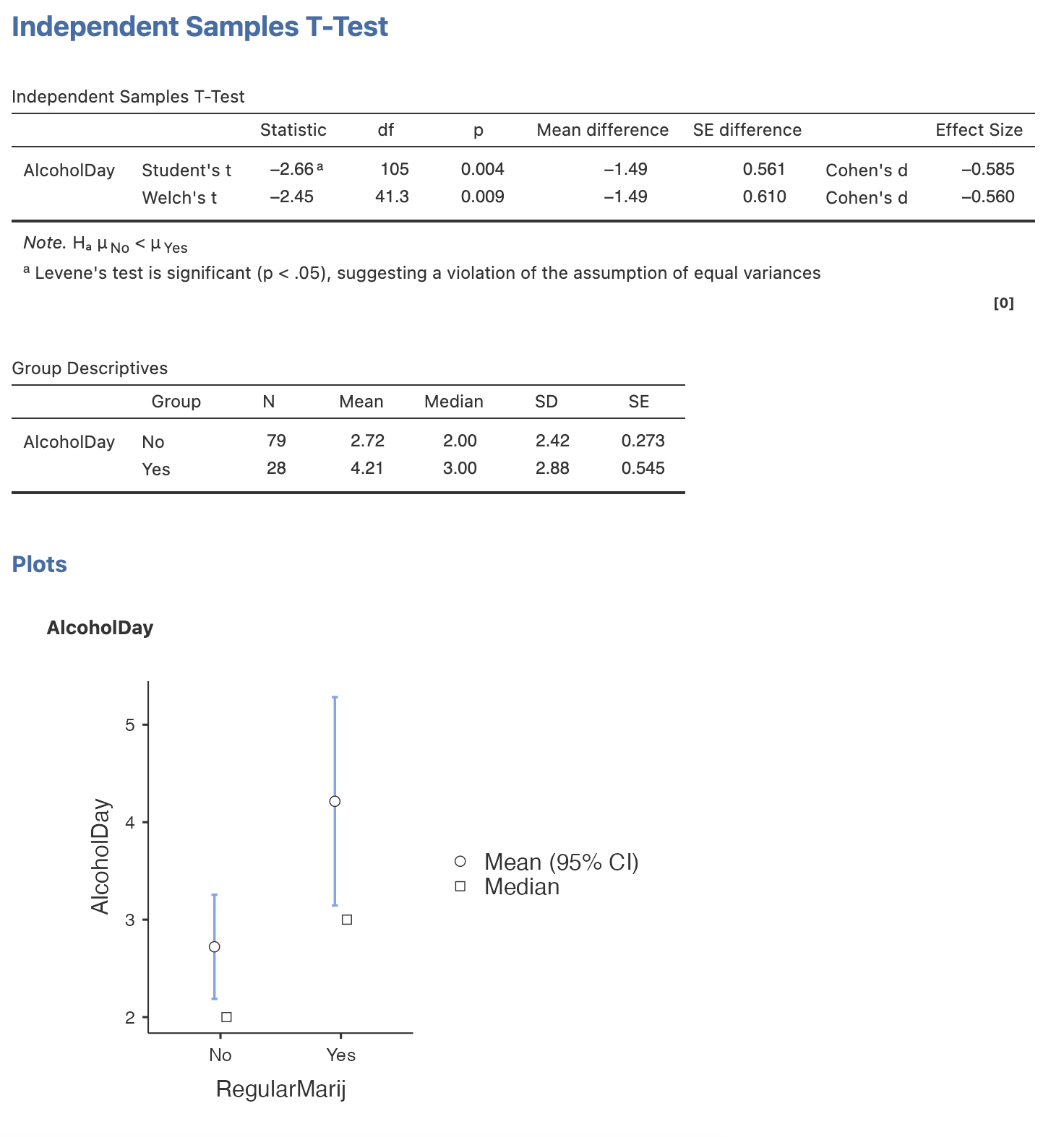
We can also conduct the Student’s t-test to assess differences between two groups of independent observations, as we discussed in an earlier chapter. As a recap, we assess the mean differences using the t-distribution. To calculate the degrees of freedom for this test, we will use the Welch test given that the group sample size differs (e.g., non-regular smokers, n = 79 versus regular smokers, n = 28). We also use the Welch test if our data violates the assumption of homogeneity of variances. We can check this in jamovi by selecting the “Homogeneity test” under Assumption Checks.
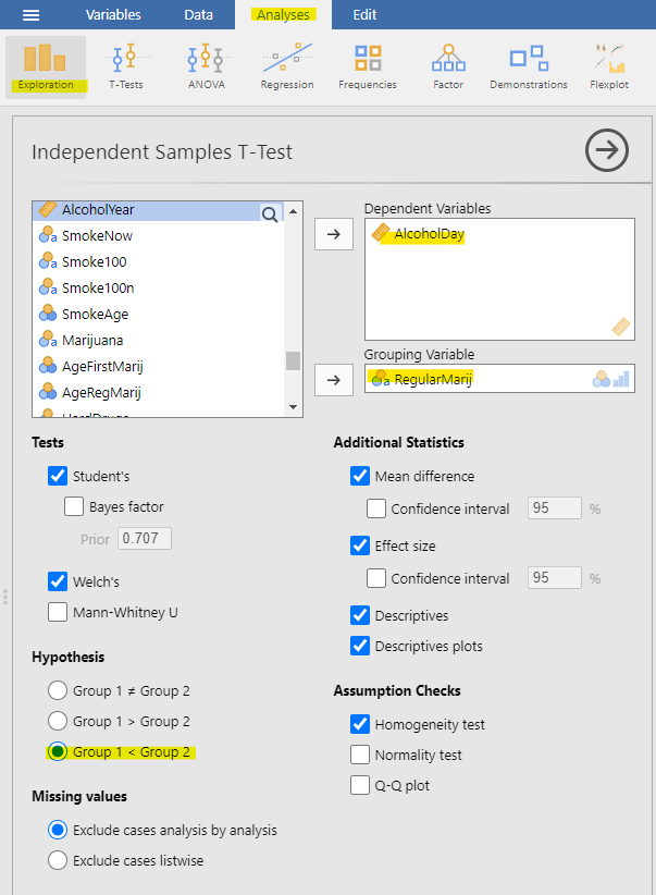
To perform the independent t-test in jamovi, follow these steps: Go to Analyses > Exploration > Place “AlcoholDay” in the dependent variables and “RegularMarij” in the Grouping Variable. As you’ve learned from previous chapters, we also want jamovi to provide us with effect size and descriptives. In this particular scenario, we began with a specific hypothesis that smoking marijuana is linked to increased alcohol consumption, so we’ll use a one-tailed test. Under Hypothesis, select “Group 1 < Group 2,” taking into account that the grouping in the “RegularMarij” variable is: 1 = No | 2 = Yes.
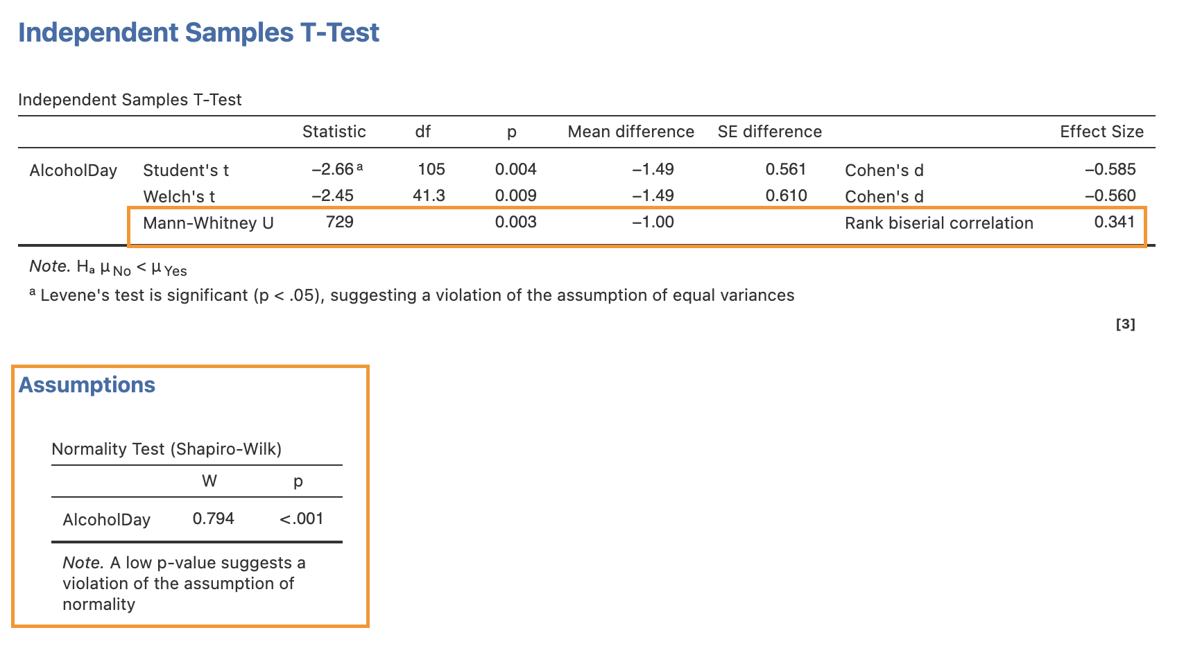
Here are the results from jamovi. We observe a statistically significant difference between the groups, as we hypothesised. Individuals who smoke marijuana are more likely to consume larger amounts of alcohol during the day.
Non-Parametric Independent t-Test: Mann-Whitney U
The t-test relies on the assumption that the data comes from populations with normal distributions. When dealing with small sample sizes, it can be challenging to rigorously assess this assumption. Instead of assuming that our data was sampled from normal populations, we can use the non-parametric Mann-Whitney test to assess differences between the two groups. Most statistical software can provide this test.
In jamovi, you can find this option within the independent samples t-test window. To check if our data violates the normality assumption, click on the “Normality test” under Assumption Checks. After performing the Shapiro-Wilk test, it appears that our data indeed violates the normality assumption, as indicated by the significant p-value.
Using the Mann-Whitney U test, we obtained a p-value of 0.003, which remains statistically significant.
The t-Test as a Linear Model
The t-test is often presented as a specialised tool for comparing means, but it can also be viewed as an application of the GLM. In this case, the model would look like this:

Dummy coding
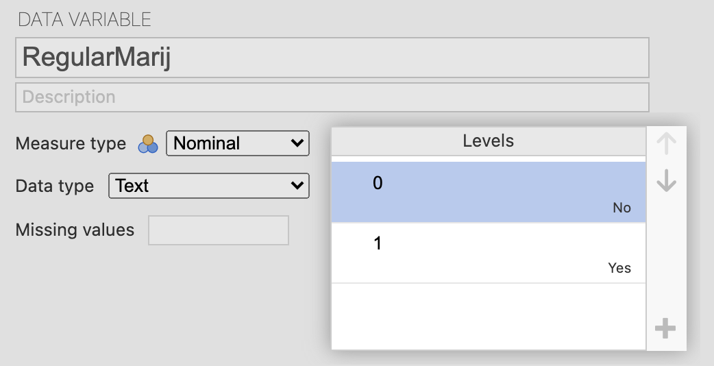
Since regular use of marijuana is a binary variable, we need to assign dummy coding to the levels of the variable. We will use 0 for non-regular users and 1 for regular users. We do this by going into double-clicking the variable you want to dummy code. This will open the data variable tab and type 0 for those who said no, and 1 for those who said yes.
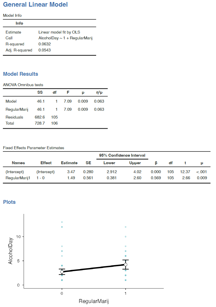
In that case, β1 is simply the difference in means between the two groups, and β0 is the mean for the group that was coded as zero. We can fit this model using the general linear model function in our statistical software. To do this in jamovi, you have to install the module named gamlj. As you can see in Figure 7.3.7 below, it will give the same t statistic above (without the Welch correction).
Comparing Paired Observations
In experimental research, we often use within-subjects designs, in which we compare the same person on multiple measurements. The measurements that come from this kind of design are often referred to as repeated measures. For example, in the NHANES dataset blood pressure was measured three times. Let’s say that we are interested in testing whether there is a difference in mean systolic blood pressure between the first and second measurements across individuals in our sample.
We see that there does not seem to be much of a difference in mean blood pressure (about one point) between the first and second measurements. First let’s test for a difference using an independent samples t-test, which ignores the fact that pairs of data points come from the the same individuals.
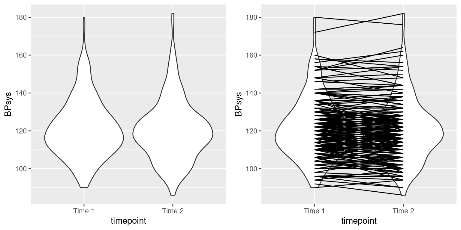
This analysis shows no significant difference. However, this analysis is inappropriate since it assumes that the two samples are independent, when in fact they are not, since the data come from the same individuals. We can plot the data with a line for each individual to show this (see the right panel in Figure 7.3.8).
In this analysis, what we really care about is whether the blood pressure for each person changed in a systematic way between the two measurements, a common strategy is to use a paired t-test, which is equivalent to a one-sample t-test for whether the mean difference between the measurements within each person is zero. We can compute this using our statistical software, telling it that the data points are paired. With this analysis, we see that there is in fact a significant difference between the two measurements.
Comparing More than Two Means
Often we want to compare more than two means to determine whether any of them differ from one another. Let’s say that we are analysing data from a clinical trial to see the efficacy of drugs in improving mood. In the study, volunteers are randomized to one of three conditions: anxifree, joyzepam or placebo. Our hypothesis is to see whether there is a significant difference in mood improvement between these three conditions. For this scenario, let’s use sample data from jamovi’s data library titled “Clinical Trial”. Let’s create a box plot for each drug with mood gain as our outcome variable (see Figure 7.3.9):
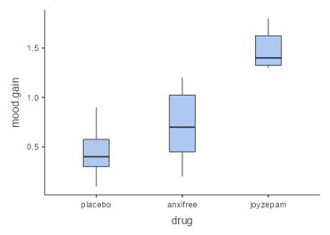
Just from looking at the box plots above, there did seem to be differences between the groups. However, let’s see if these differences are statistically significant.
Analysis of Variance
We would first like to test the null hypothesis that the means of all of the groups are equal – that is, neither of the treatments had any effect compared to placebo. We can do this using a method called analysis of variance (ANOVA). This is one of the most commonly used methods in psychological statistics, and we will only scratch the surface here. The basic idea behind ANOVA is one that we already discussed in the chapter on the general linear model, and in fact, ANOVA is just a name for a specific version of such a model.
We can partition the total variance in the data (SStotal) into the variance that is explained by the model (SSmodel) and the variance that is not (SSerror). We can then compute a mean square for each of these by dividing them by their degrees of freedom:


Where k is the number group means we have computed.
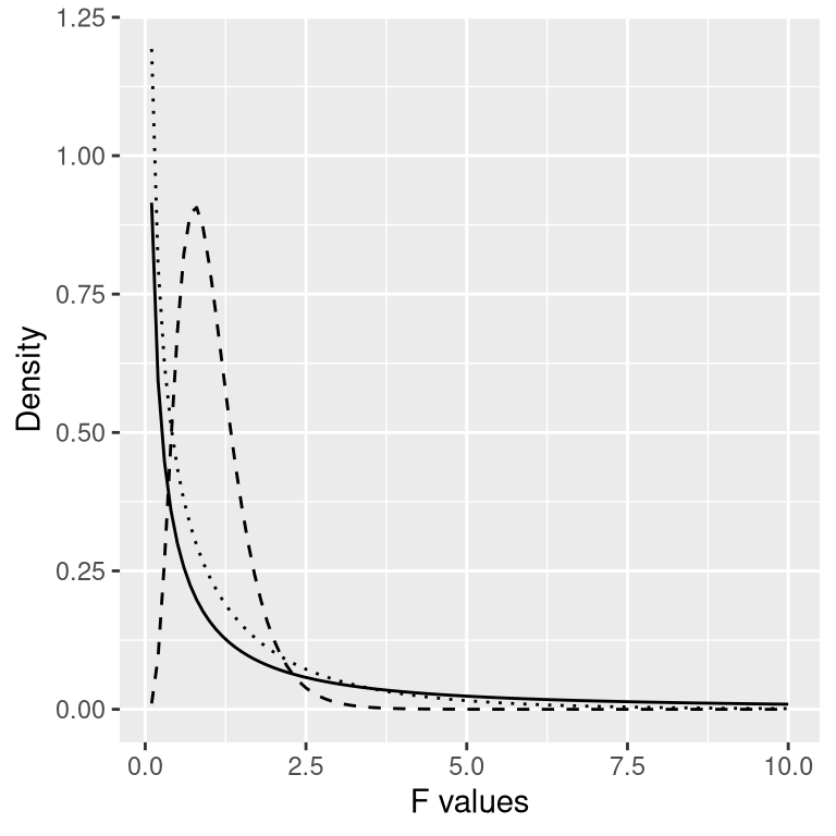
With ANOVA, we want to test whether the variance accounted for by the model is greater than what we would expect by chance, under the null hypothesis of no differences between means. Instead of the t-distribution, we use another theoretical distribution that describes how ratios of sums of squares are distributed under the null hypothesis: The F distribution (see Figure 7.3.10). This distribution has two degrees of freedom, which correspond to the degrees of freedom for the numerator (which in this case is the model), and the denominator (which in this case is the error).
To create an ANOVA model, we extend the idea of dummy coding that you encountered earlier. Remember that for the t-test comparing two means, we created a single dummy variable that took the value of 1 for one of the conditions and zero for the others. Here we extend that idea by creating three dummy variables, one that codes for placebo (i.e., 0) and 1 for anxifree and 2 for joyzepam. We can then use the ANOVA function to determine if there are differences between the three groups.
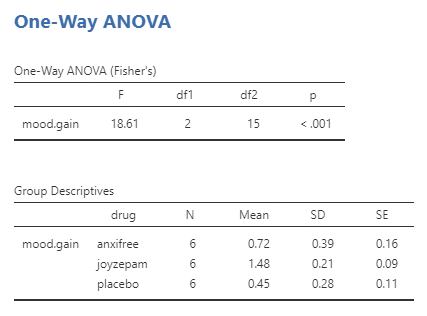
Remember that the hypothesis that we started out wanting to test was whether there was any difference between any of the conditions; we refer to this as an omnibus hypothesis test, and it is the test that is provided by the F statistic. In this case, we see that the F test is significant (p-value is < 0.001), consistent with our impression that there did seem to be differences between the groups. However, the output does not specifically inform us which of the drugs significantly differs from the placebo and by how much. If we believe that one of the drugs is not significantly different from the placebo, would it not make more sense to opt for the placebo?
We can ask jamovi to provide more tests for us. Post-hoc tests can be conducted to delve deeper into the differences between each drug and the placebo. These tests can offer a more granular understanding of the comparative effects. By utilising additional post-hoc tests in jamovi, we can enhance the precision of our analysis and make more informed decisions regarding the potential efficacy of each drug compared to the placebo.
Why not Multiple t-Tests?
Let’s use the example we have above: anxifree, joyzepam and placebo. We might think of doing three separate t-tests: comparing anxifree to joyzepam, anxifree to placebo and joyzepam to placebo.
But, we don’t do multiple t-tests because it increases the chance of making a Type I error. If I did three separate t-tests, set my alpha (Type I error rate) at 5% for each, and knew for sure there’s actually no effect, each test has a 5% chance of making a Type I error. But since we’re doing three tests, our overall error rate becomes 14.3%, not the 5% we set alpha at.
With more tests, it gets riskier:
- 1 test: 5%
- 2 tests: 9.8%
- 3 tests: 14.3%
- 4 tests: 18.6%
- 5 tests: 22.6%
- 10 tests: 40.1%
- 20 tests: 64.1%
So, doing 10 tests could have a 40% chance of showing a false positive (saying there’s an effect when there isn’t). To avoid this, we use one-way ANOVA as one test to see if there’s a difference overall. We can also do things to control our error rate. Check out this xkcd comic for a good visual explanation.
Post-Hoc and Planned Comparisons
Post-Hoc Comparisons
Sometimes, we want to know not just if there’s a difference overall (which the F-statistic tells us), but where exactly the differences are between groups. To figure that out, we use planned contrasts when we have specific ideas we want to test or post-hoc comparisons when we don’t have specific ideas. It’s important to mention that you only do these comparisons if the ombinus F-statistic is statistically significant. There’s no point in looking at differences between groups if the test says there are no differences between the groups!
Here are some details about post-hoc comparisons:
- No correction: This doesn’t correct for errors at all, like doing separate t-tests for each group. It’s not recommended because it can mess up our error rate (as discussed above).
- Tukey: This is a common one. It controls errors well but isn’t as strict as Bonferroni. The p-values are smaller than unadjusted but not as big as Bonferroni.
- Scheffe: It’s complicated, and I don’t use it much.
- Bonferroni: This is super conservative, good if you don’t have many comparisons or really want to control errors. It multiplies your p-value by the number of comparisons.
- Holm: Like Bonferroni but adjusts p-values sequentially, making it less strict.
Remember, if you’re doing Welch’s F-test (unequal variances) or Kruskal-Wallis test (non-normal distribution), use the Games-Howell or DSCF pairwise comparisons, respectively.
Planned Comparisons
If you already have specific ideas about differences between groups before analyzing your data, you’d use planned contrasts. You can find these in the ANOVA setup as a drop-down menu. Just a heads up, you can’t do planned contrasts with Welch’s F-test or Kruskal-Wallis test.
Even though there are six contrasts in jamovi, you usually only do one. Here they are for explanation:
- Deviation: Compares each category (except the first) to the overall effect. The order is alphabetical or numerical. Placebo is considered the first category (because I have manually put this in the first level).
- Simple: Compares each category to the first. The order is alphabetical or numerical. Placebo is considered the first.
- Difference: Each category (except the first) is compared to the mean effect of all previous categories.
- Helmert: Each category (except the last) is compared to the mean effect of all subsequent categories.
- Repeated: Each category is compared to the last.
- Polynomial: Tests trends in the data. It looks at the n-1th degree based on the number of groups. For example, with 3 groups, it tests linear (1) and quadratic (2) trends. If there were 5 groups, it would test linear (1), quadratic (2), cubic (3), and quartic (4) trends. Note: Your factor levels must be ordinal for a polynomial contrast to make sense.
Running ANOVA as a GLM
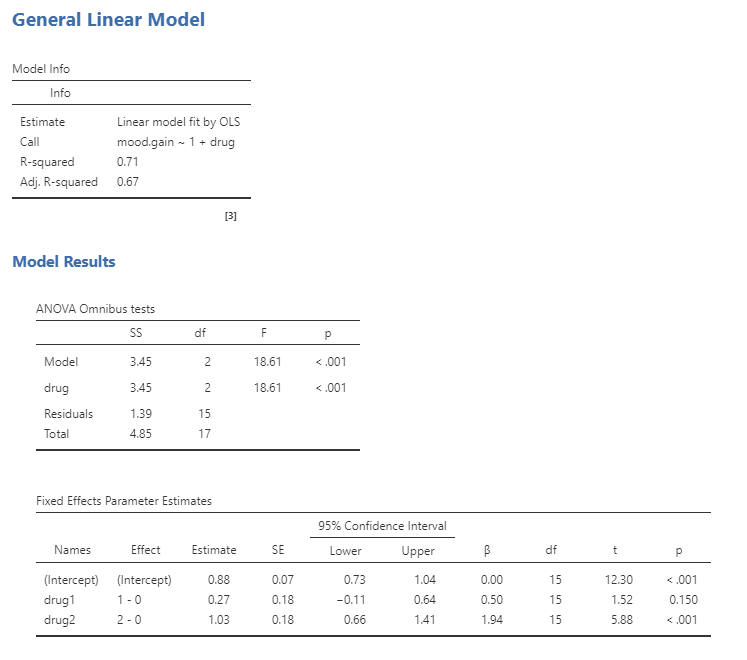
We can also just run ANOVA as a GLM using the methods above. Using GLM, jamovi will also provide the ANOVA omnibus tests and you will see that the F test is identical to the ANOVA method. GLM will also provide us with the result of a t-test for each of the conditions, which basically tells us whether each of the conditions separately differs from placebo; it appears that Drug 2 (joyzepam) does whereas Drug 1 (anxifree) does not. However, keep in mind that if we wanted to interpret these tests, we would need to correct the p-values to account for the fact that we have done multiple hypothesis tests (otherwise, we are inflating our error).
Chapter attribution
This chapter contains material taken and adapted from Statistical thinking for the 21st Century by Russell A. Poldrack, used under a CC BY-NC 4.0 licence.
Screenshots from the jamovi program. The jamovi project (V 2.2.5) is used under the AGPL3 licence.
