6.4 The Central Limit Theorem

The following video shows the Galton box in action. It is a device used to illustrate the principles of probability and the Gaussian distribution, which is often referred to as the normal distribution or bell curve. As you can see, seemingly random events of balls being released will accumulate into the bottom forming a bell-shaped curve. This visual device shows how randomness can lead to predictable patterns when many random events are combined. This also demonstrates the idea of regression to the mean.

Most importantly, it also demonstrates the central limit theorem (CLT), which states that, with enough sample size, the data will approximate to a normal distribution, regardless of the original distribution of those variables.

The normal distribution is described in terms of two parameters: the mean (which you can think of as the location of the peak), and the standard deviation (which specifies the width of the distribution). The bell-like shape of the distribution never changes, only the location of the peak and width. The normal distribution is commonly observed in data collected in the real world – and the central limit theorem gives us some insight into why that occurs.

Let’s use a module available within jamovi to understand how central limit theorem works. Under Modules, install CLT – Demonstrations. This is a simple jamovi module that contains simulations to help students visualise important lessons in probability, such as how the law of big numbers and how central limit theorem work. Students can also use this module to visualise correlations of different sizes and grasp important concepts when testing hypotheses.

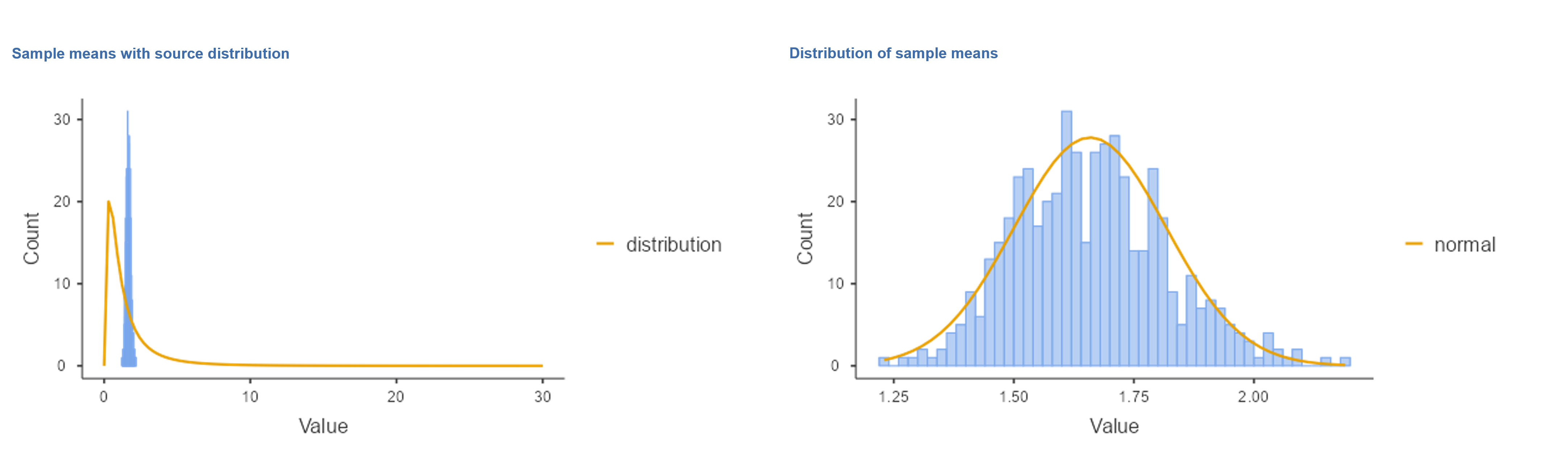
Under this module, we can see how central limit theorem works by looking at different sources of distribution (e.g., normal, uniform, lognormal, etc.) and how the distribution of the sample means can lead to a normal distribution if the sample is large enough. For example, the right panel in Figure 6.4.1 shows the source distribution which has a lognormal shape. Lognormal distributions are commonly seen in variables such as the population’s wealth when the data is skewed to the right. In other words, the distribution has a long tail towards the right.

Now, let’s look at the sampling distribution of the mean for this source distribution (left panel in Figure 6.4.1). This graph was simulated by repeatedly drawing 500 trials from the source distribution and taking the mean. Despite the clear non-normality of the original data, the sampling distribution is remarkably close to the normal.

The central limit theorem is important to understand because it allows us to safely assume that the sampling distribution of the mean will be normal in most cases. This means that we can take advantage of statistical techniques that assume a normal distribution. It’s also important because it tells us why normal distributions are so common in the real world: any time we combine many different factors into a single number, the result is likely to be a normal distribution. For example, the height of any adult depends on a complex mixture of their genetics and experience — when we get enough data on height, the resulting distribution of the data will be in a bell-shaped curve.