5.5 Variability: How Spread Out are the Values?
Once we have described the central tendency of the data, we often also want to describe how variable the data is – this is sometimes also referred to as dispersion. In other words, we want to how widely dispersed the data is as it helps us make sense of the data we have.
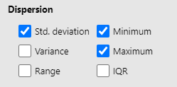
Let’s say that we’ve gathered data on the heights of 250 university students in a statistics subject and also the heights of a sample of 250 professional basketball players from Australia’s National Basketball League. Let’s assume that the average height for both groups is about 170 centimetres.
Using the descriptive statistics we’ve discussed so far, you might initially think that the heights of the university students and the basketball players are quite similar. However, this is not the case. Anyone who’s ever watched a basketball game would notice that those basketball players look like they all have the same height – otherwise, shorter players may be disadvantaged given that basketball is known as the sport for the “giants”.[1]
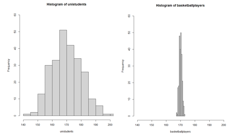
While both groups have approximately the same “average” height, the university students have a much broader range of heights around that midpoint, indicating that their heights vary more and extend further from the middle. In contrast, the basketball players might all appear to have similar heights, making the heights of the uni students seem more diverse. To put it as simply as possible, if all our collected scores were found to be the same, there would be no variability. The more different the values collected are, the more variability there is.
This dispersion in height is an important characteristic when describing these two groups because it allows us to quantify precision and uncertainty.
Variance and Standard Deviation
So, let’s dive into our dataset of university students’ heights to explore how we can measure this variation. For simplicity’s sake, let’s just look at 5 of the student heights. The table below displays these heights in centimetres and how much their heights deviate from the mean height:
Table 5.5.1. Student heights in centimetres and how much their heights deviate from the mean height
| Student Height (cm) | Height Deviation from Mean (cm) |
| 165 | – 5 |
| 170 | 0 |
| 175 | 5 |
| 180 | 10 |
| 185 | 15 |
We call the second column deviations. These deviations show how far each student’s height is from the mean height.
Now, let’s compute the average deviation or the average distance by which a student’s height deviates from the mean. We start by summing the deviation scores:

At first glance, it might seem like, on average, students’ heights deviate by 25 centimetres from the mean, which doesn’t make much sense.
However, here’s where the magic of statistics comes into play. The positive and negative deviations cancel each other out, leading to an average of zero. This outcome highlights a critical point: deviations (or differences from the mean) always sum to zero. So, we’re stuck at this point.
But, there’s a clever solution. What if we compute the average of the absolute values of the deviations? Let’s try it:

35 divided by the number of students (5) gives us an average deviation of 7 centimetres. This makes sense and tells us that, on average, a student’s height deviates by about 7 centimetres from the mean height.
However, this is not the standard deviation; when we compute the standard deviation, we don’t use absolute values. Instead, we square the deviations. So, let’s calculate the average of the squared deviations:

The square root of 350 is approximately 18.71 centimeters. This is the standard deviation, and it tells us that, on average, a student’s height deviates by about 18.71 centimetres from the mean height.
In summary, understanding dispersion in the context of university students’ heights helps us measure how much individual heights vary from the average. It’s not just about the average height; it’s about the range of individual heights, and the standard deviation is a valuable tool for quantifying this variation.
Range
Range is another measure of variable in the data. The range is the difference between the lowest score and the highest score – the largest value minus the smallest value. For example, we may have a scale with a possible scoring range of 1 to 50.
However, it is also possible that no one in the sample scored higher than 40. Therefore, we have a “theoretical” range (i.e., the possible range) and the “actual range” (i.e., the range we actually got when we collected the data).
The interquartile range (IQR) is like a “fence” that encloses the middle portion of your data. It is calculated as the difference between the third quartile (the 75th percentile) and the first quartile (the 25th percentile). It helps us understand how tightly or loosely packed the data is, while ignoring outliers.
Available measures of variability in jamovi
Under Analyses > Exploration, you will find the available measures of variability in jamovi
Homogeneity of Variance
Homogeneity of variance (also known as homoscedasticity) is an important concept in statistics, particularly when we are comparing two different groups or examining relationships between two different variables. It can be a difficult name to say, but it’s not a difficult concept to comprehend. Homogeneity comes from the word homogenous – meaning “same”. Therefore, it refers to the idea that the variability (or spread) of data points should be roughly the same across different groups or levels of the variables.
Let’s go back to the example above regarding the heights of university students and basketball players, as you can see in Figure 5.5.1, the basketball players’ heights are tightly clustered together (low variance), and university students’ heights are scattered widely (high variance). In this example, we do not have homogeneity of variance. This makes it challenging to draw meaningful conclusions because the variability within groups is not consistent.
If, instead, we compared the heights of university students and the heights of teachers, then it is more likely that the heights are spread out fairly evenly within each group. In other words, the spread of scores would be fairly homogenous. It is easier to compare the groups because you don’t have one group with extremely tightly clustered scores and another with widely dispersed scores.
Homogeneity of variance is important because it ensures that the assumptions of various statistical tests are met (which we will learn more later on). When the assumption of homoscedasticity is violated, it can affect the validity and reliability of the results. To address this, researchers might need to use data transformation techniques or different statistical methods designed to handle unequal variances.
Chapter attribution
Screenshots from the jamovi program. The jamovi project (V 2.2.5) is used under the AGPL3 licence.
- Although it is important to note that there are great basketball players who are less than 6 feet (or 183 cm). For an entertaining read: https://www.theguardian.com/sport/2022/nov/15/nba-basketball-height-tall-players-advantages ↵
