Example 5.5
Design of shallow foundations at the Ultimate Limit State using numerical methods
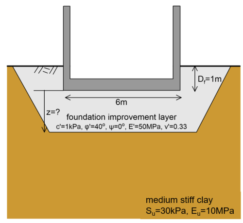
A storage facility with dimensions 6 m x 30 m will be founded on a mat foundation i.e., a slab, that for practical purposes can be consider as an infinite strip footing. The embedment depth of the foundation cannot exceed Df = 1 m, for practical reasons. The foundation subsoil consists of a medium stiff saturated clay layer, with the properties depicted in the figure below. Preliminary calculations resulted in short-term bearing capacity qf = 180 kPa, which is lower than the ultimate limit state pressure provided by the Structural Engineer 200 kPa.
As the dimensions of the footing are fixed on the geometry of the facility, improvement measures must be implemented. The Geotechnical Engineer proposed the replacement of the clay with coarse-grained well-compacted material, as the most cost-effective ground improvement solution. Determine the minimum required thickness of the improvement layer to increase the bearing capacity to acceptable levels (qf > 200 kPa), while taking into account the following:
- Consider for simplicity the unit weight of both the clay and the foundation improvement layer to be equal to γ = 18 kN/m3.
- Do not apply any reduction factors on the shear strength of the geomaterials as per Eq. 5.33 and 5.34, nor a geotechnical strength reduction factor on the bearing capacity.
- Assume the footing to be rigid and rough.
Answer:
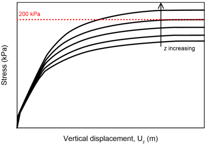
Determining the optimum thickness of the foundation improvement layer is a trial-and-error procedure. We are seeking to find the thickness that will result in a bearing capacity slightly higher than 200 kPa (Figure 5.43); not too high, because that would mean that the solution is not economical.
We will thus assume different thickness for the improvement layer, considering rather crude increments of e.g., 0.5 m, and get the load-settlement curve from different PLAXIS models. Notice that employing Eq. 5.35 while assuming a friction angle for the foundation improvement layer φ′ = 40º results in a critical thickness of the foundation improvement layer for the failure to be constrained in it:


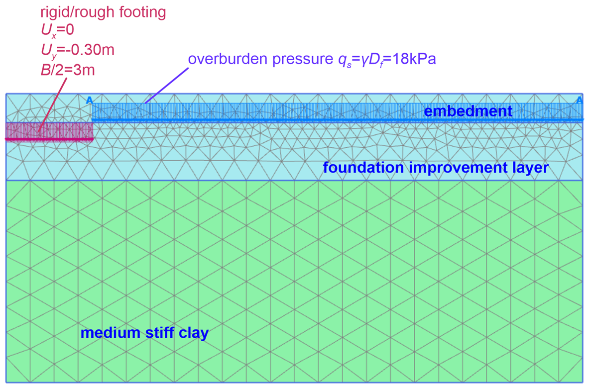
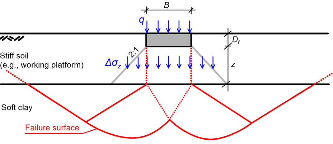
This implies that we definitely have to consider the soft clay layer in our numerical model, and account for the possibility of punching failure, according to the mentioned in Section 5.5.3. We will simulate a plane-strain geometry of 20 m x 10 m, with the axis of the footing being an axis of symmetry (Figure 5.44). The top cluster of the geometry corresponds to the embedment depth (to be replaced by an equivalent pressure), the middle to the foundation improvement layer, and the bottom to the clay. The extent of the model should be enough to accommodate the complex failure surface illustrated in Figure 5.38a.
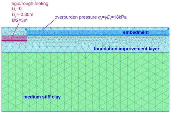
A prescribed displacement is applied to simulate the rigid and rough footing loading at the foundation level. As discussed in Example 5.2, the vertical displacement Uy should be enough to reach the collapse load i.e., Uy = -0.30 m. Additionally, applying Ux = 0.0 m along the width of the footing accounts for the rough interface i.e., no horizontal displacement is allowed to develop. To simulate embedment, we apply a uniform pressure outside the model area occupied by the footing, with magnitude equal to the weight of the excavated soil, as in Example 5.2:

We are seeking to determine the short-term bearing capacity. As presented in Table 5.4, the coarse-grained improvement material, which is usually a mixture of sand with gravels, will behave as drained, whereas the saturated fine-grained clay will behave as undrained under short-term loading conditions. As we are not interested in estimating excess pore pressure but only the bearing capacity, and no groundwater table is present, we will perform a total stress analysis TSA. For that we will use the Mohr-Coulomb Drained model to simulate the improvement material, and the Mohr-Coulomb Undrained (C) model to simulate soft clay’s response (see also Example 5.2), with the shear strength and compressibility properties presented in the problem definition. Keep in mind that undrained or drained response refers to material behavior, so the same problem may include different materials behaving as drained or undrained under short term loads, depending on their properties.
The dilation angle of the improvement layer is assumed ψ = 0o. We will use the Davis equivalent shear strength parameters c* and φ* (Eqs. 5.5-5.7) together with associative flow to model the response of this layer, and compare the outcomes to the analytical solution described in Section 5.5.3 to investigate whether the use of Davis parameters provides reasonable estimates of the bearing capacity. Eqs. 5.5-5.7 yield:


where 
The analysis is performed in two stages. During the initial stage before the construction of the footing, geostatic stresses are initialized with the “K0 procedure”, considering all the three clusters depicted in Figure 5.44 as active, whereas the prescribed displacement and the uniform pressure qs are not active. When the prescribed displacement load is activated, at the subsequent plastic step, the top soil cluster is deactivated, as discussed in Example 5.2, and the pressure qs is activated.
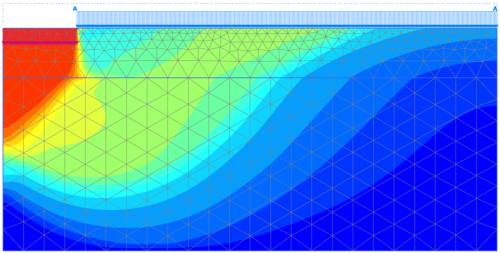
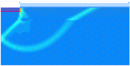
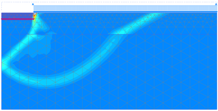
Results of the analysis for thickness of the foundation improvement layer z = 2 m are presented in Figure 5.45, in terms of the geometry of the developing failure surface. The shape of the failure surface depicted in Figure 5.45 is similar to the theoretical failure surface presented in Figure 5.38a, and suggests that “punching” of the footing indeed takes place, with failure developing within the soft clay layer.
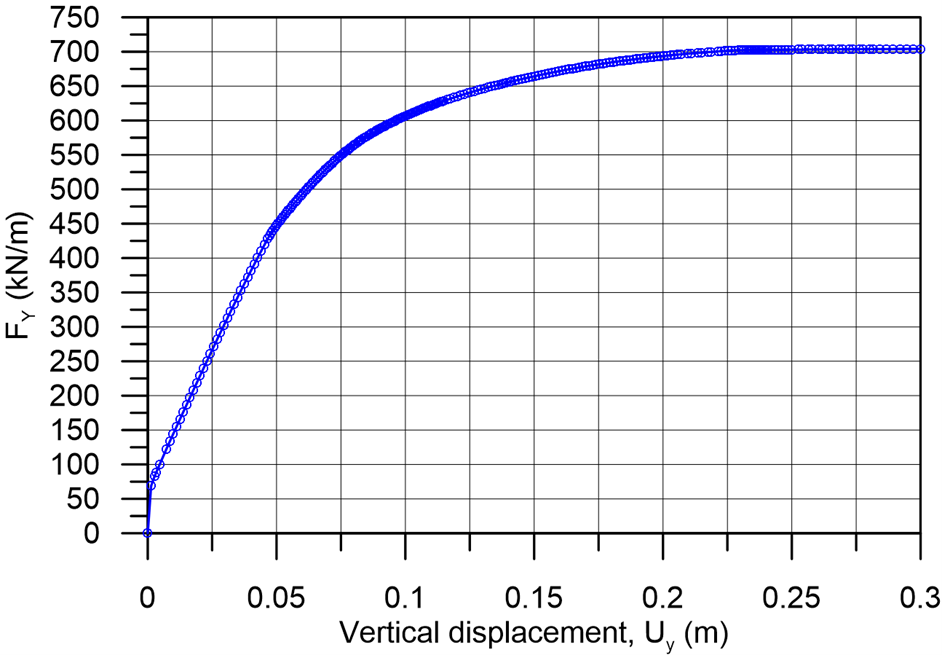
The force-settlement curve used to define the collapse load of the footing is presented in Figure 5.46. In a plane-strain problem, the reaction force is provided in PLAXIS in kN/running meter of the strip footing. As we are simulating only half of the footing geometry, referring to the load-settlement curve of Figure 5.46 the bearing capacity will be:
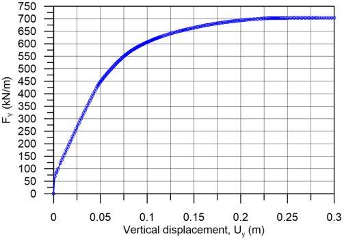

thus higher than the ultimate limit state pressure (200 kPa). The total reaction force on the 6m-wide footing is equal to 2xFY =1408 kN/m.
Replacement of 2 m of clay below the foundation level with coarse-grained material resulted in ≈ 60 kPa increase in the bearing capacity (about 35%). Yet, it is considerably higher than the required bearing capacity of 200 kPa. The optimum improvement layer thickness that will result to bearing capacity marginally higher than the ultimate limit state pressure from the structure can be determined via a parametric analysis, trying different thickness z values, thus analyzing different model geometries.
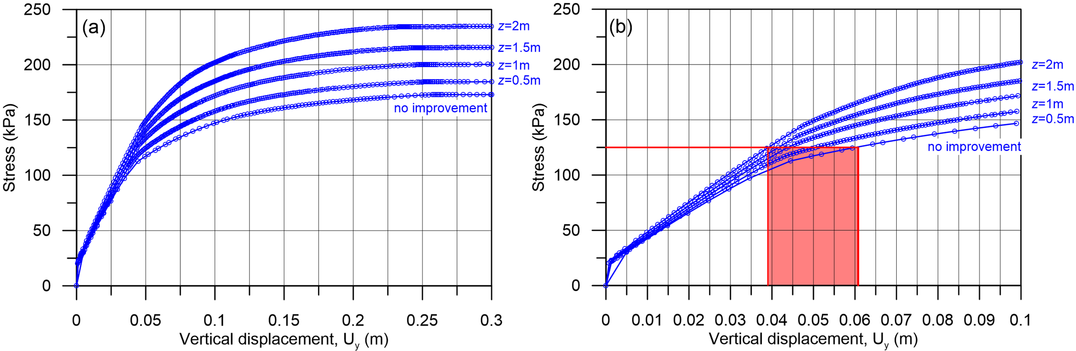
From Figure 5.47, where the results of analyses for different z values are presented in terms of load-settlement curves, we conclude that an improvement layer with thickness z = 1 m is enough to increase the bearing capacity to 200 kPa.
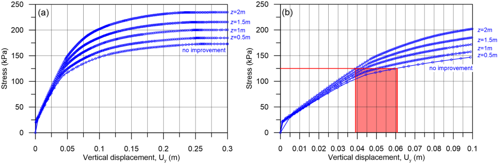
Notice in Figure 5.47a that the bearing capacity develops for settlement values higher than about 0.20 m, a value that is (most probably) not acceptable under serviceability conditions. If we zoom into lower stress levels where serviceability stress is most likely to lie in (Figure 5.47b), we observe that the improvement layer plays a two-fold role: it increases the bearing capacity, but also reduces the settlement for a given applied pressure.
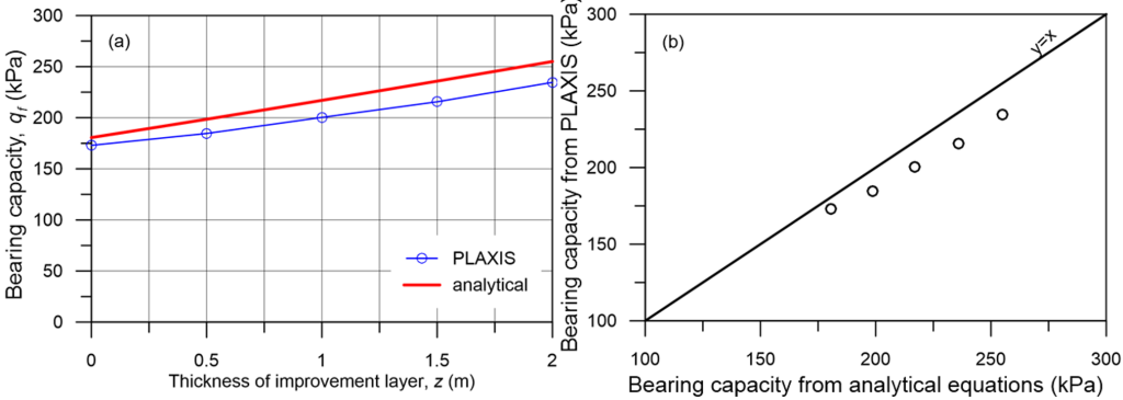
The same problem can be solved analytically too, using the approximate methodology presented in Section 5.5.3 and in Example 5.4 (see Additional Problem 5.10.1). Results of the analytical methodology, in terms of bearing capacity for variable thickness of the compressive layer, compare well with the numerical results (Figure 5.48), suggesting that i) the approximate methodology can be effectively used for practical problems, at least during preliminary design stages, and ii) use of the Davis effective shear strength parameters together with an associated flow rule yields comparable results.
