Example 5.2

Use PLAXIS to confirm the value of the collapse load found analytically in Example 5.1 (Q_f = 942.5×2.5² = 5890 kN). Repeat the comparison for the case where the embedment depth of the footing is D_f = 2 m.

Answer:

The radius of the footing has been estimated with the analytical method, so the geometry of the axisymmetric problem is fully defined (Figure 5.15a). Using PLAXIS, we can find the load-settlement curve for the particular footing diameter. The collapse load Q_f is the reaction for which settlement increases without any increase in the applied load (Figure 5.15b).

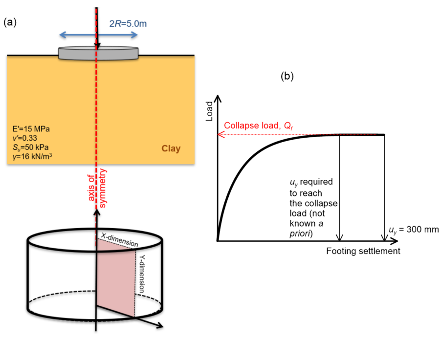
As we are interested in determining the short-term bearing capacity of a footing on clay, we have to consider undrained response according to Section 5.2.5, and perform a total stress analysis. Keep in mind that the water table level does not play any role in a total stress analysis, as failure is defined in terms of total stresses. Employing the Undrained (C) Mohr-Coulomb model, we have to input the undrained shear strength provided in Figure 5.15 S_u = 50 kPa, as well as the undrained Young’s modulus of the soil, calculated from Eq. 4.11 as:

The undrained Poisson’s ratio of the soil is automatically set by PLAXIS equal to v_u ≈ 0.5, and accounts for the fact that no volume change takes place under undrained loading conditions i.e., the undrained bulk modulus of the soil K_u = E_u/3(1-2v_u) is practically infinite. Note here that v_u cannot be taken equal to v_u = 0.5 in PLAXIS, and a value of e.g., v_u = 0.495 is used instead, to prevent a division-by-zero in the calculation of the bulk modulus.

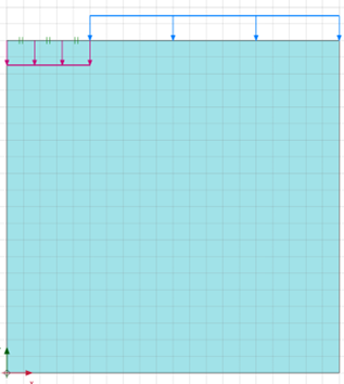
A square 10 m x 10 m slice is used to simulate the problem, which should be more than enough to accommodate the failure surface that is expected to develop as the load on the footing approaches the collapse load. Recall that here our aim is to determine the maximum load that the footing can safely carry, not the settlement of the footing. Thus, the location of the bottom boundary can be within the influence depth of the applied pressure on the model surface, provided that the failure surface is accommodated within the soil slice. The settlement estimates in that case however will not be accurate, as a “shallow” fixed bottom boundary will lead to underestimation of settlement for a given applied pressure value.

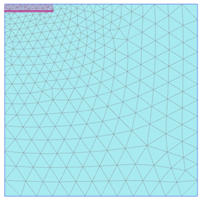
The finite element mesh created while considering “medium” global coarseness is shown in Figure 5.16. A prescribed displacement is applied along the footing radius to simulate loading of a rigid and rough footing, as discussed in Example 4.2. The vertical displacement U_y should be enough to reach the collapse load i.e., the load-displacement curve should reach an asymptote (Figure 5.15b). A value of U_y = -0.30 m should be enough for that, for the particular compressibility parameters considered. Additionally U_x = 0.0 m along the radius of the rough footing.

Analysis is performed in two stages: The “K₀ procedure” is used to initialise geostatic stresses, and subsequently the prescribed displacement simulating loading of the footing up to failure is activated in a single “plastic” loading step.

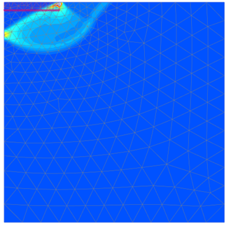
Results of the analysis are presented in Figure 5.17, in terms of shear strain increments developing in the soil around the footing at failure, when the applied displacement has reached U_y = -0.30 m. Notice that the geometry of the failure surface that develops compares well will the log-spiral surface that was assumed while calculating analytically the bearing capacity.

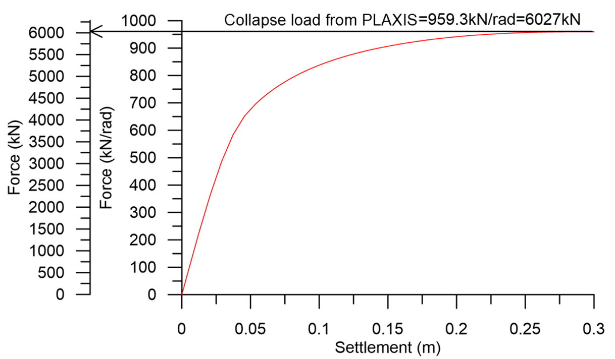
The force-displacement curve can be obtained by considering a node at the footing axis, and plotting the reaction force F_Y versus the vertical displacement (settlement) of the same node U_y (Figure 5.18).

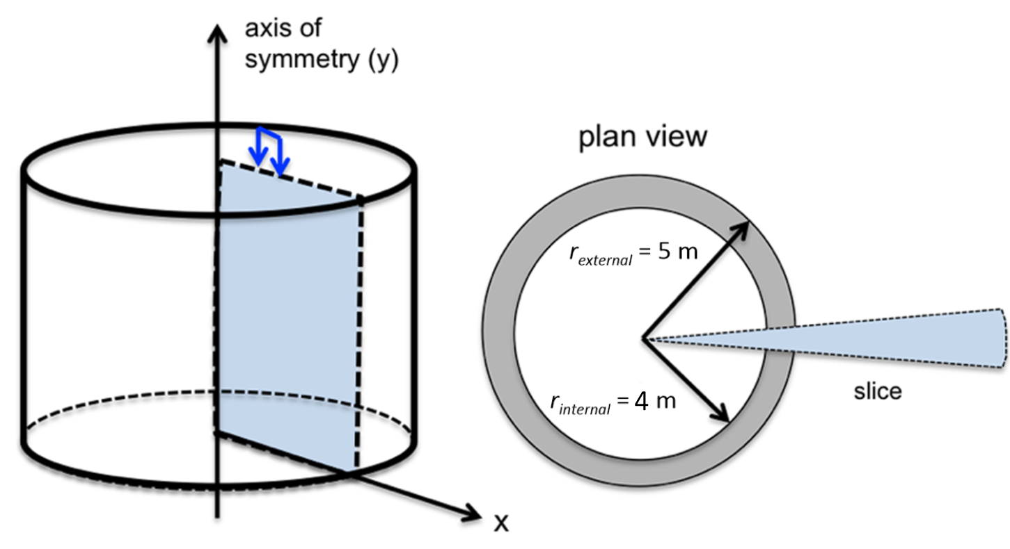
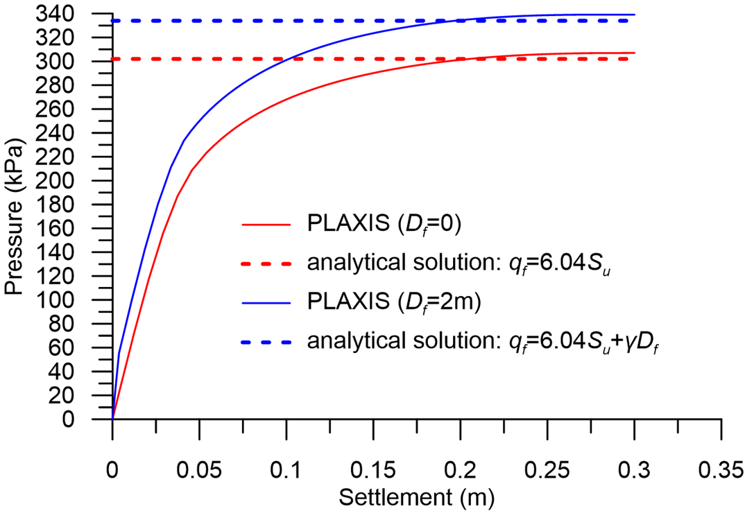
As discussed in Example 4.2, the reaction force is provided by PLAXIS in kN/rad, since we are simulating a “slice” of the problem of angle 1 rad (see also Figure 3.17). The total reaction force at failure, which corresponds to the plateau of the curve, will be 959.3 kN/rad x 2π = 6027 kN, and the bearing capacity in terms of stress will be 6027/(πR²) = 307 kPa; very close to the analytical solution from Example 5.1 (red continuous and dashed lines in Figure 5.19).

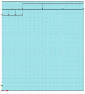
A similar model is prepared for the case of the footing embedded at depth D_f = 2 m. To simulate the effect of embedment, we define two geometry clusters in PLAXIS, with the top cluster having a thickness equal to the embedment depth (Figure 5.20). Subsequently we apply a prescribed displacement to simulate loading of the footing at the foundation level, while outside the model area that corresponds to the footing, we apply a uniform pressure with magnitude equal to the weight of the excavated soil:

where γ = 16 kN/m³ is the unit weight of the excavated soil. Initialisation of geostatic stresses with the “K₀ procedure” is performed with both geometry clusters active, while the prescribed displacement and the uniform pressure q_s are not active. When the loading (prescribed displacement) is applied on the footing, at the subsequent plastic phase, the top cluster is deactivated. Deactivation of a geometry cluster in PLAXIS suggests that this part of the soil is excavated. At the same time, both the prescribed displacement and the pressure q_s are activated in the model. The soil pressure around the footing represents the non-excavated soil outside its perimeter (Figure 5.20). This is an efficient way of simulating footing embedment, and was also used for the derivation of the analytical expressions provided in Example 5.1. As one may notice from the results presented in Figure 5.19, again the numerically estimated bearing capacity in terms of stress q_f = 339 kPa compares well with the results of the analytical solution for a rough circular footing (blue continuous and dashed lines in Figure 5.19):