Example 4.6

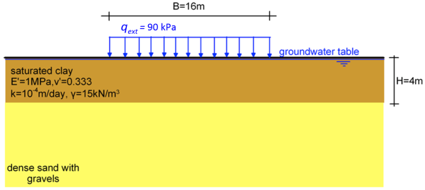
Calculate the degree of consolidation of the compressible clay layer depicted in the figure below a) 100 days, and b) 5 years after the application of an infinite strip pressure. Consider the bottom layer of dense sand with gravels to be incompressible and permeable. Compare the settlement below the center of the pressure at t = 5 years with the settlement estimated analytically in Example 4.3.

Answer:

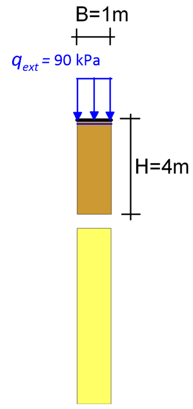
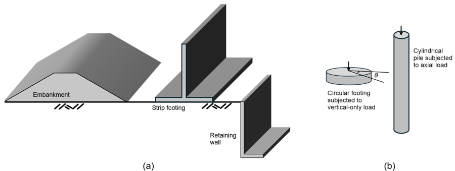
As discussed in Example 4.3, we can assume 1-D consolidation conditions, given that the width of the loaded area is large, compared to the thickness of the compressible clay layer. This suggests that we do not need to simulate the full two-dimensional problem: a 1m-wide soil column (unit cell) would suffice, provided that the correct boundary conditions are applied (Figure 4.43). Note that the width 1 m is arbitrary, results are independent of the selected width of the unit cell, provided that pressure is applied across the entire width of the unit cell. As the strip pressure extents “infinitely” along the out-of-plane dimension, the problem will be simulated as plane-strain (Figure 3.4a).

As also discussed in Chapter 4.8, for the simulation of consolidation we also have to account for permeability boundary conditions, on top of displacement boundary conditions (Figure 4.44). “Standard fixities” in PLAXIS will apply the necessary displacement boundary conditions for the plane-strain problem. As the bottom layer of dense sand with gravels is incompressible, we can choose not to explicitly introduce it in the model, and fix the displacement at the bottom of the clay layer in both directions (Figure 4.44). Thus the dimensions of the model will be 1 m x 4 m.

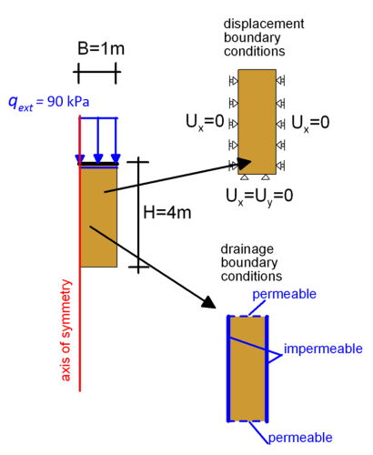
“Permeable” boundary conditions are applied at the top and bottom of the clay layer to specify that water is free to flow from these directions. “Impermeable” boundary conditions at the lateral boundaries account for symmetry and for vertical-only water flow. Note that the axis of symmetry always corresponds to impermeable boundary conditions. The considered boundary conditions ensure that lateral strains will be zero ε_x = ε_h = 0 and that excess pore water pressure dissipates only vertically.

The undrained (A) linear elastic model is used to simulate clay behaviour under the applied loading, which allows for the calculation of (excess) pore water pressures in plastic stages. Compressibility is defined in terms of effective parameters i.e., the drained Young’s modulus E′ and Poisson’s ratio v′. Note however that the undrained behavior stiffness parameters (E_u, v_u = 0.495) are calculated internally by PLAXIS, and the coefficient of earth pressure at-rest K₀ is automatically set equal to K₀ = 1. Note that in PLAXIS we do not input v_u = 0.50, but a value very close to 0.5. That it because the (undrained) bulk modulus of soil K_u = E_u/3(1-2v_u) becomes infinite if v_u = 0.50 (soil is incompressible), resulting in a division-by-zero. The permeability of the clay, k is also entered as a material parameter.

The analysis consists of three stages:

• Step 1: Initial phase. The geostatic stresses and hydrostatic pore water pressures before the application of the external pressure are initialised with the “K₀-procedure”. Drainage boundary conditions and groundwater table level are defined, as in Figure 4.44.
• Step 2: Sudden application of the loading. A “Plastic” step is introduced, where the external pressure is instantaneously applied on the ground surface i.e., the duration of this step (time interval) is 0.0 days.
• Step 3: Consolidation. A “Consolidation” step follows the previous plastic step, where the external pressure will remain on the ground surface for a prescribed time interval, and excess pore pressures developed during Step 2 will be allowed to dissipate through the free-draining boundaries. “Reset displacements to zero” should not be active, so that any immediate settlement will be co-estimated.

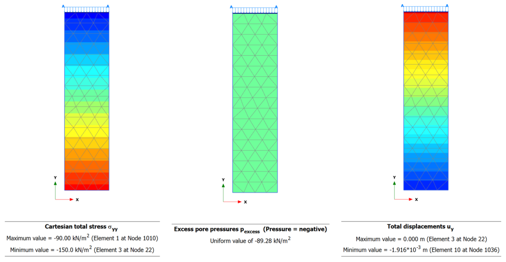
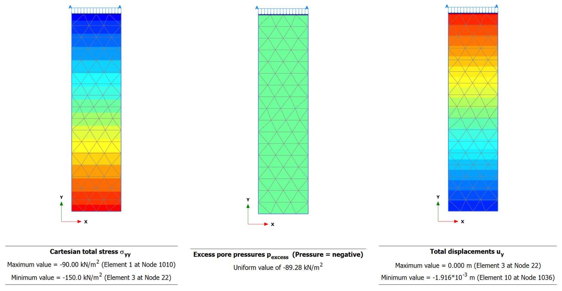
Results at the end of Step 2 are presented in Figure 4.45 in the form of contours of total vertical stress along the thickness of the clay layer, excess pore pressure distribution, and settlement. Notice that excess pore water pressures are not equal to the external applied pressure as you might expect, but somewhat lower, and some immediate settlement develops. This is because PLAXIS considers a large, yet realistic bulk modulus for water, unlike the analytical solution where we assumed that water is incompressible.

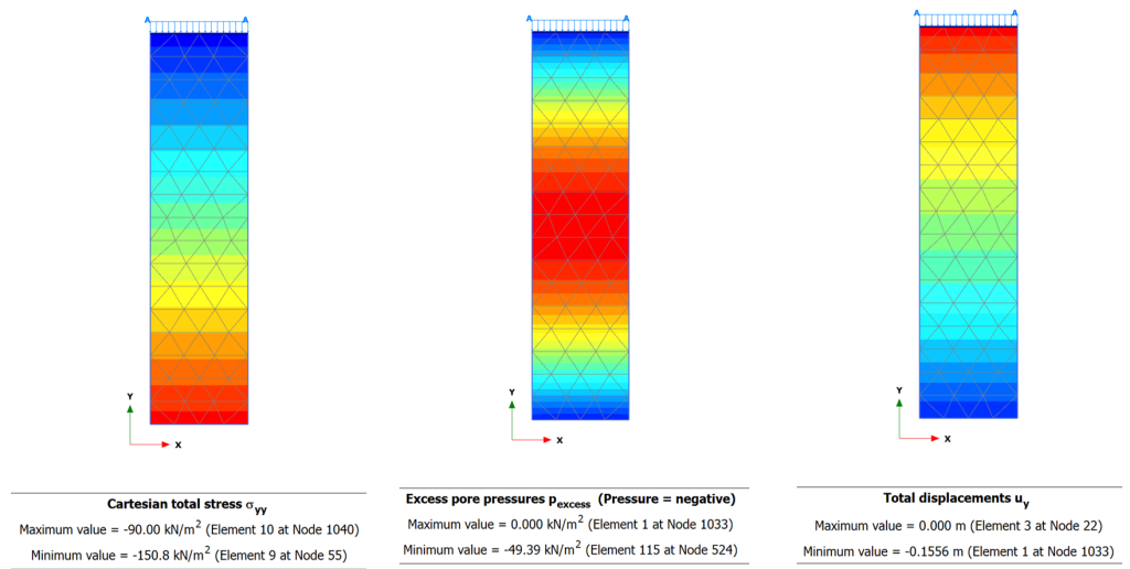
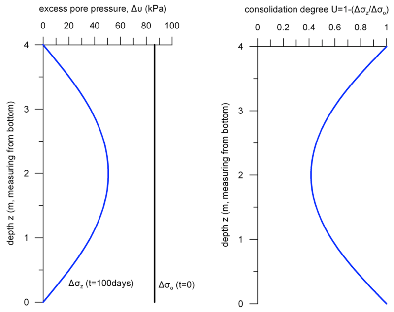
Results at the end of Step 3, after t = 100 days, are presented in Figure 4.46, again in terms of total vertical stress, excess pore pressure distribution and settlement contours, for comparison. As expected, total stresses do not change. Excess pore water pressures have partly dissipated, but the maximum value at the middle of the sample is Δu = 49.4 kPa (Figure 4.47) which suggests that consolidation has not been completed yet (U < 100 %), and settlement has not attained its maximum value. Notice also in Figure 4.47 that excess pore pressure at the top and bottom boundary, where drainage is free, is zero.

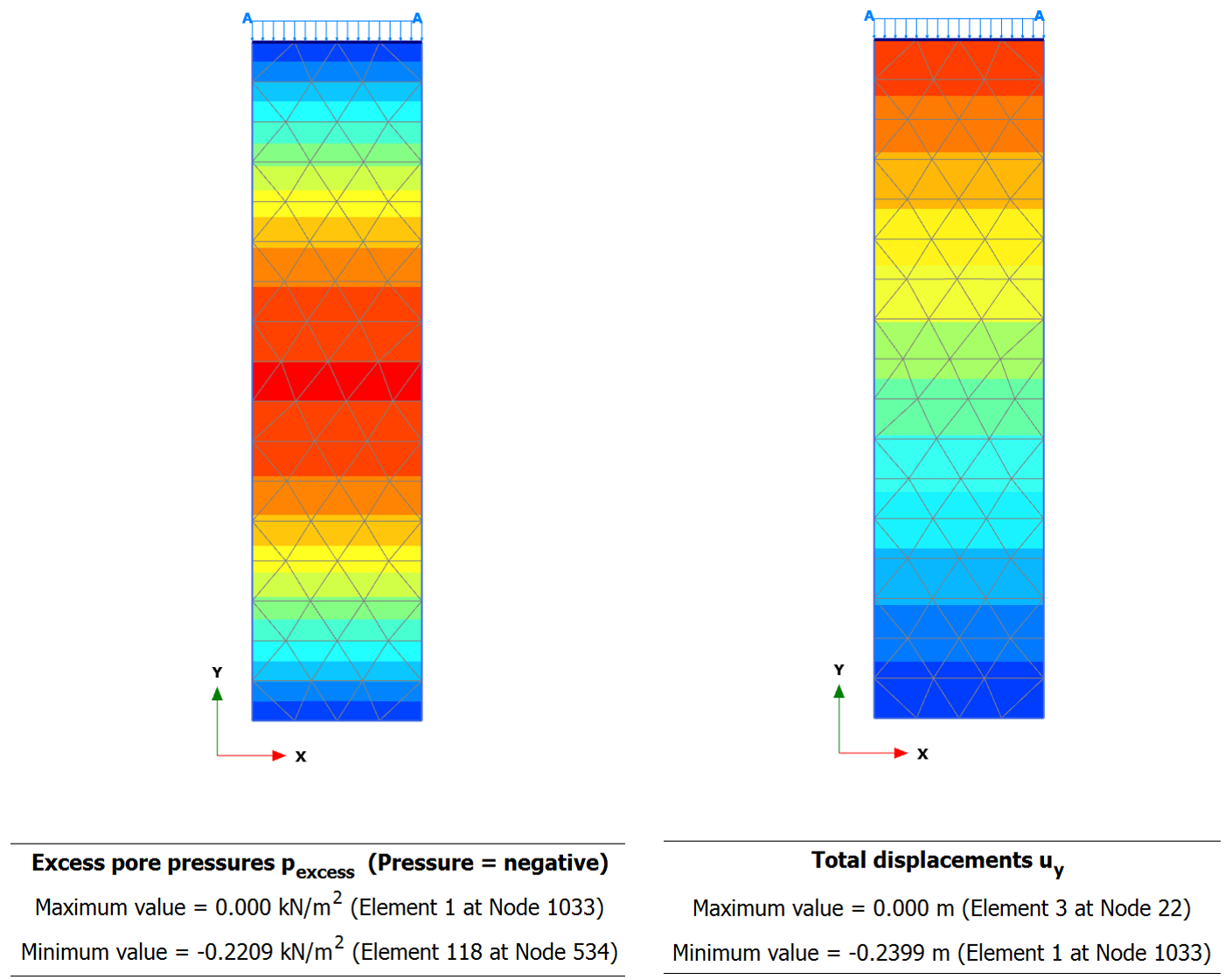
If Step 3 is run for t = 1825 days (5 years), excess pore pressure will become practically zero along the full thickness of the clay (Figure 4.48a), which implies that consolidation has been completed, and the full primary consolidation settlement has developed (Figure 4.48b).

Total stresses will of course remain unchanged. The degree of consolidation will be equal to U ≈ 100% along the thickness of the soil layer. The value of settlement is, as expected, practically equal to the value computed analytically in Example 4.3 (ρ_pc = 240 mm).