Example 4.4
Estimation of a 1-D primary consolidation settlement using the results of an oedometer test
Calculate again the primary consolidation settlement due to the strip pressure, using this time the oedometer test results depicted in the figure.
Answer:
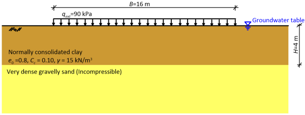
As discussed in Example 4.3, the width of the loaded area is large, compared to the thickness of the compressible layer so we can well assume 1-D consolidation conditions. The additional effective stress Δσ′z due to the application of the pressure will be equal to the applied pressure Δσ′z = qext = 90 kPa.
To improve accuracy when the problem involves rather thick compressible layers (H > 2 m) and we are using non-linear consolidation theory, we can divide the layer into sublayers, and find the settlement of each sublayer (Figure 4.33) separately.
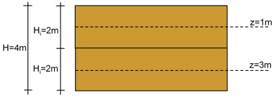
Accordingly, we sum individual settlements to find the settlement of the entire compressible layer. In the corresponding equations, H will be the thickness of each sublayer (Hi), and the effective stresses will be calculated at the middle of each sublayer.
As the clay is normally consolidated, we will apply Eq. 4.34 for the estimation of the settlement of each sublayer. The necessary calculations are presented in the table below:
| Geostatic total stress σz0 = γz | Hydrostatic pore pressure u0 = γwz | Geostatic effective stress σ′z0 = σz0 – u0 | Final effective stress σ′fin = σ′z0 + qext | log(σ′fin/σ′z0) | Settlement of each sublayer, ρpc | |
|---|---|---|---|---|---|---|
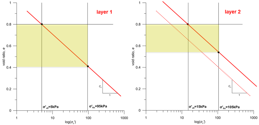
| Sublayer 1 (Hi = 2m) | 15 kPa | 10 kPa | 5 kPa | 95 kPa | 1.278 | 0.14 m |
| Sublayer 2 (Hi = 2m) | 45 kPa | 30 kPa | 15 kPa | 105 kPa | 0.845 | 0.09 m |
| Total settlement: | 0.23 m | |||||
As expected, settlement of sublayers 1 and 2 is not equal, as the preconsolidation stress (equal in this case to the initial, geostatic effective stress as the clay is normally consolidated) increases with depth, while the applied pressure on both is 90 kPa. This is illustrated in the figure below, where the path followed by a soil element at the middle of each sublayer is presented, and is a consequence of introducing soil non-linear response in consolidation calculations.