Example 4.2
Numerical estimation of the load-settlement curve of a footing resting on a sand layer
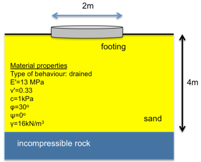
Estimate the load-settlement curve of the circular footing illustrated below, for settlement up to 30 mm. Consider sand to behave as elastic-perfectly plastic, obeying the Mohr-Coulomb failure criterion. Assume the footing is: a) rigid and rough and b) flexible, made of reinforced concrete with thickness h = 0.2 m.
Answer:
As sand behavior is drained, total settlement will develop immediately after the application of the loading (Section 4.4), thus we do not need to consider the time factor in this analysis. Contrary to the method for determining immediate settlement described in Section 4.5.4, in this analysis the compressible sand layer has a limited thickness of 4 m, while it is assumed to behave non-linearly when loaded. While it is not common to assume non-linear soil response in serviceability analysis, we do so here to introduce the reader to non-linear finite element analyses, and their intricacies. A short description of the Mohr-Coulomb material model implemented in PLAXIS can be found in Section 5.2.5, and the reader can refer to it if not familiar with the elastic-perfectly plastic material model obeying the Mohr-Coulomb failure criterion.
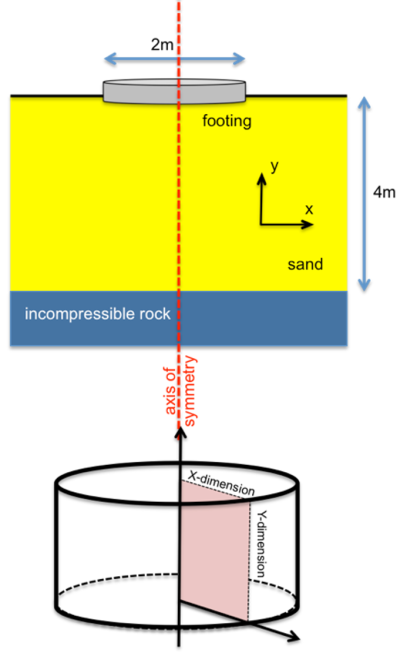
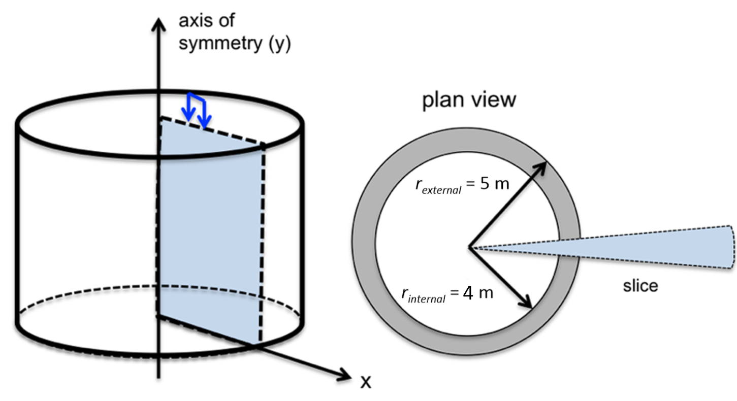
The problem is axisymmetric, with the axis of symmetry passing through the center of the footing, as depicted in Figure 4.18. Only half of the footing is hence simulated.
The underlying rock layer will not be simulated. Instead, we will fix the displacements of the bottom boundary of the sand layer in both directions, which is essentially the same as considering an incompressible layer at that elevation. Thus, a 5 m x 4 m rectangular geometry would suffice for the simulation of this problem. Setting the lateral boundary to be at a distance of 5 times the footing radius from the axis of symmetry is a rational first-order approach. However, it is imperative to check the sensitivity of the model results to the distance of the area of interest from the lateral boundaries.
Standard fixities are applied, to account for symmetry along the left lateral boundary, and also fix the displacement along both directions at the bottom boundary, as discussed above.
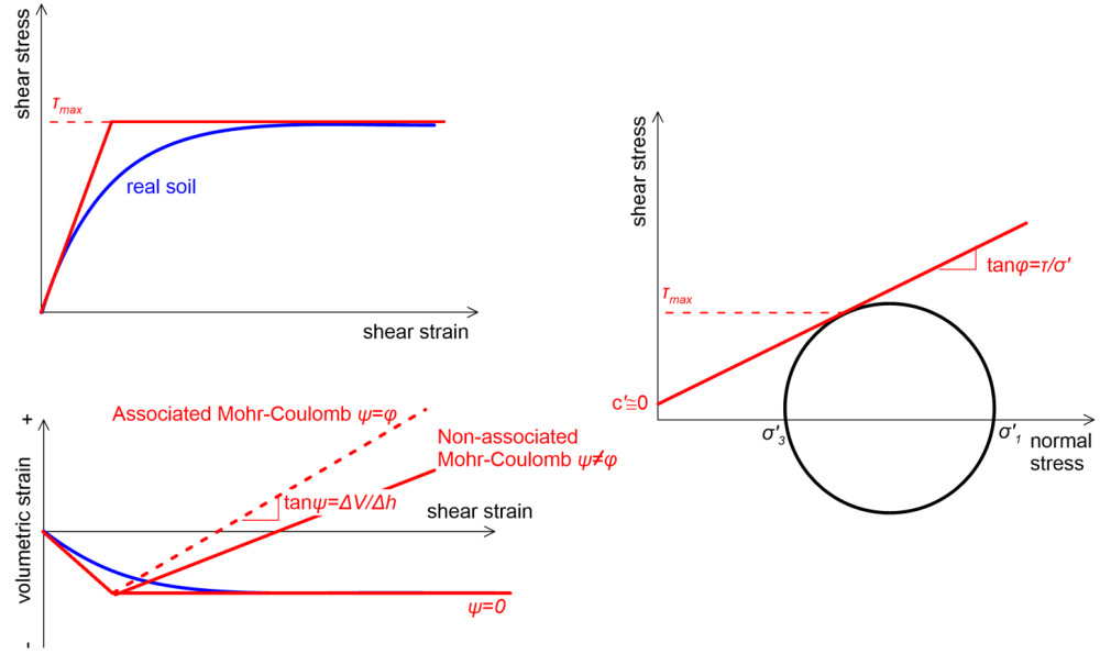
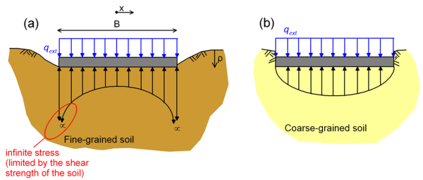
Sand response is simulated with the Mohr/Coulomb-Drained material, using effective stress shear strength and compressibility parameters (Figure 4.19). High-permeability coarse-grained materials behave as drained under both short-term and long-term load conditions. Note that clean sands generally do not exhibit cohesion (c′ = 0). However we use a small value c′ ≤ 1 kPa to avoid simulating a material of zero strength at the surface of the model (y = 0), for numerical stability reasons. Such a small cohesion value does not affect the results we are interested in. This is further discussed in Part 5.
Notice also that we consider the dilation angle ψ, which controls the amount of volumetric sand deformation that takes places as shear strains increase to failure, to be equal to ψ = 0. This implies that at failure shearing takes places under constant volume, whereas some contraction (compression) will take place under elastic conditions (Figure 4.19). The simulated response is compatible with experimental tests in loose sands (and normally consolidated clays). On the other hand, the friction angle φ′ = 30 deg controls the maximum (failure) shear stress that the soil can carry under the current normal stress.
When the dilation angle is considered equal to the friction angle ψ = φ′ then the flow rule of the Mohr-Coulomb model (which controls the amount of volumetric deformation at failure) is called “Associated” whereas when the dilation angle attains any other value ψ ≠ φ′ is called “Non-associated” (Figure 4.19). Note that (unlike metals) the assumption of associated flow for soils is in contradiction with experimental data, as it will overestimate the amount of volumetric deformation that takes place during shearing. Hence the use of non-associated flow rule (i.e., a realistic dilation angle) will result in perhaps better approximation of the deformation behaviour. However, this also causes a number of numerical issues (localisation phenomena, non-uniqueness of the collapse load, poor convergence), even when techniques such as the “Arc-length” method are used to solve the system of non-linear equations (instead of Newton-Raphson methods), which is a good choice when the stiffness matrix is not a positive definite i.e., when softening is expected. A more detailed discussion on this is, however, beyond the scope of this Chapter. A technique to avoid such issues is again described in Part 5. Since we simulate serviceability conditions here, such issues should not affect the analysis, as yielding (failure) of soil elements will be limited.
The “rigid” footing will settle uniformly (Figure 4.10), implying that the vertical displacement Uy be constant along the radius of the footing. Moreover, since the rigid footing is also assumed to be “rough”, no slippage will occur at the soil-footing interface, and the horizontal displacement Ux will be zero along the radius of the footing. In other words, we do not need to simulate the actual footing using structural elements, but we can replace it by a set of prescribed displacements acting along its radius:
- Ux = 0 to prohibit slippage at the soil-footing interface (“rough” footing)
- Uy = -0.03m to calculate the load-settlement curve up to a settlement of 30 mm (“rigid” footing)
Notice that the desired outcome from this analysis is the complete load-settlement curve, not settlement for a specific load. In fact, from the load-settlement curve we can estimate settlement under any load, up to the maximum reaction on the footing that will develop for Uy = -0.03m.
Simulating a “flexible” footing by introducing in the model its actual rigidity, which depends on its geometry and material properties, is more realistic. Moreover, this analysis will also provide the internal forces developing on the footing that can be used for the structural design of the footing. This is realised in PLAXIS by adding a “plate” in the model along the radius of the footing. The properties assigned to the plate elements include:
Flexural rigidity of the footing: 
Axial rigidity of the footing: 
where h is the thickness of the footing, Ef is the Young’s modulus of the footing’s material, and vf is the Poisson’s ratio of the footing’s material. The term (1- ) in the above equations accounts for the fact that the plate elements used by PLAXIS are actually 2-D Kirchoff-Love plates and not 3-D Euler-Bernoulli beams, since we model axisymmetric or plane-strain problems. For the case at hand h = 0.2 m, Ef = 20 GPa and vf = 0.2, considering a cracked concrete section so:
EI = 13,888 kNm2
EA = 4,166,666 kN
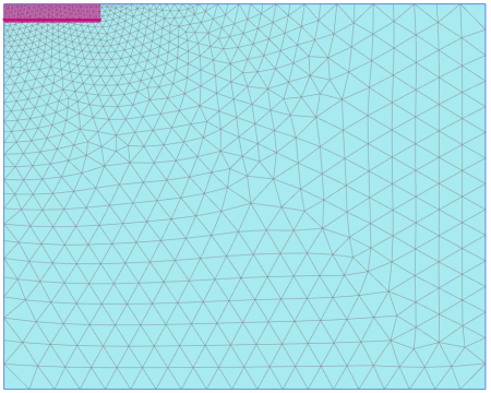
A uniformly distributed pressure is applied on the footing which, for comparison purposes, will be determined as the pressure required to achieve footing settlement equal to 30 mm with the rigid footing model. The “fine” option is used to create the finite element mesh (Figure 4.20).
Note that in the flexible footing model, use of standard fixities will also restrict in-plane rotation of the plate node lying on the axis of symmetry, and rotation of the footing at its center shall be zero. A coarse grid is used for the analysis with the flexible footing, to identify any possible mesh sizing effects on the solution.
Analysis is run in two stages. Before the application of the imposed displacement/pressure on the footing, geostatic stresses must be calculated. When the soil surface, the boundaries between soil layers, and the phreatic level (groundwater table) are all horizontal, we can invoke the so-called “K0 procedure” in PLAXIS to calculate initial geostatic stresses due to gravity. For the case at hand, with reference to the coordinate system of Figure 4.18 that follows PLAXIS nomenclature:
Vertical geostatic total stress σy0 = γy
where γ is the unit weight of the soil and y the vertical distance from the surface, and
Horizontal geostatic total stress σx0 = K0σy
where K0 is the lateral earth pressure coefficient at-rest. Effective stresses will be equal to the total stresses, as no groundwater is present. K0 can be entered manually, or calculated automatically by PLAXIS as:
- K0 = 1-sinφ‘ when the Mohr-Coulomb non-linear material model is used
- K0 = v′/(1-v′) when the linear elastic material model is used
where φ′ is the friction angle of soil, and v′ is its drained Poisson’s ratio. Subsequently a “plastic” analysis step is executed, during which the loading is activated. The deformed mesh at the end of the analysis with the rigid footing is presented in Figure 4.21a, when displacement has reached its ultimate value of 30 mm.
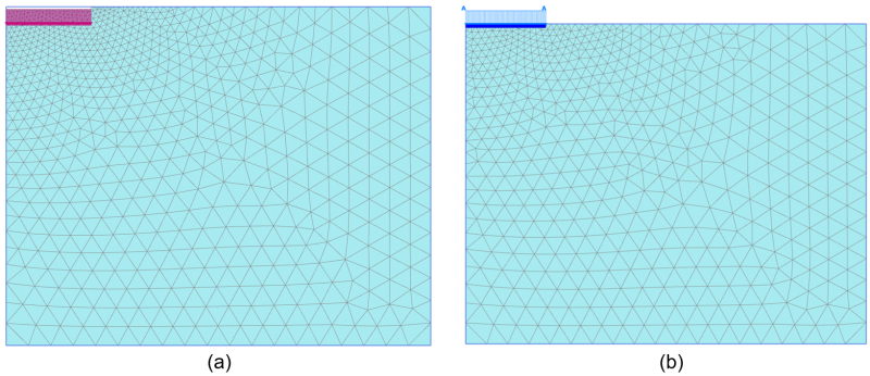
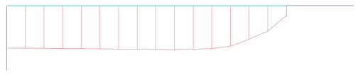
The corresponding pressure at the footing is 137.5 kPa. Note that PLAXIS provides the reaction force in axisymmetric problems in kN/rad, since we are simulating a 1-rad slice of the three-dimensional geometry (see Figure 3.17). To calculate the total reaction force, the reaction force from PLAXIS must be multiplied by 2π. The deformed mesh at the end of the analysis with the flexible footing is presented in Figure 4.21b. The deformed mesh shape is, as expected, very similar, while the ultimate settlement of the flexible footing is equal to 29 mm. Notice also that the normal stress distribution below the rigid footing, depicted in Figure 4.22, is compatible with the theoretical distribution presented in Figure 4.10b.
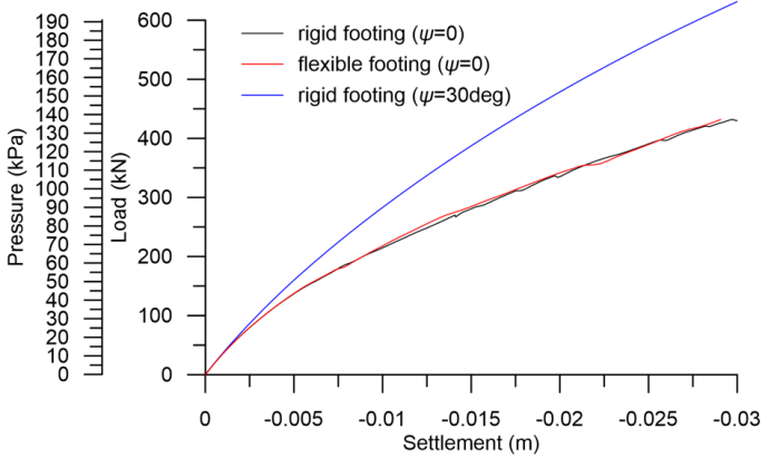
The load-settlement curves, and the comparison between the solution for the rigid footing and the flexible footing are presented in Figure 4.23. Again, as expected, both curves are very similar, implying that the effect of the rigidity of the footing on the load-settlement response is minimal in this particular problem. However, this is not the case for the effect of flow rule (dilatancy). Notice that when associated flow is considered (ψ = φ′), settlements for given loading are underestimated considerably. A detailed discussion on the causes of that are again beyond the scope of this Part. However, the reader must bear in mind that when we are simulating a material with a non-associated flow rule we introduce localisations in the solution (observable in Figure 4.23 with the form of some “oscillations” in the force-displacement curve), that result in local yielding of finite elements and reduction of the overall stiffness of the soil below the footing. Secondly, the flow rule is related with constraints in the kinematics of the shear bands formed in sand, which are minimum in the case of associated flow. As consequence, settlement under the same loading is lower.
