"

6.28 Pile group effects on the lateral load response of piles

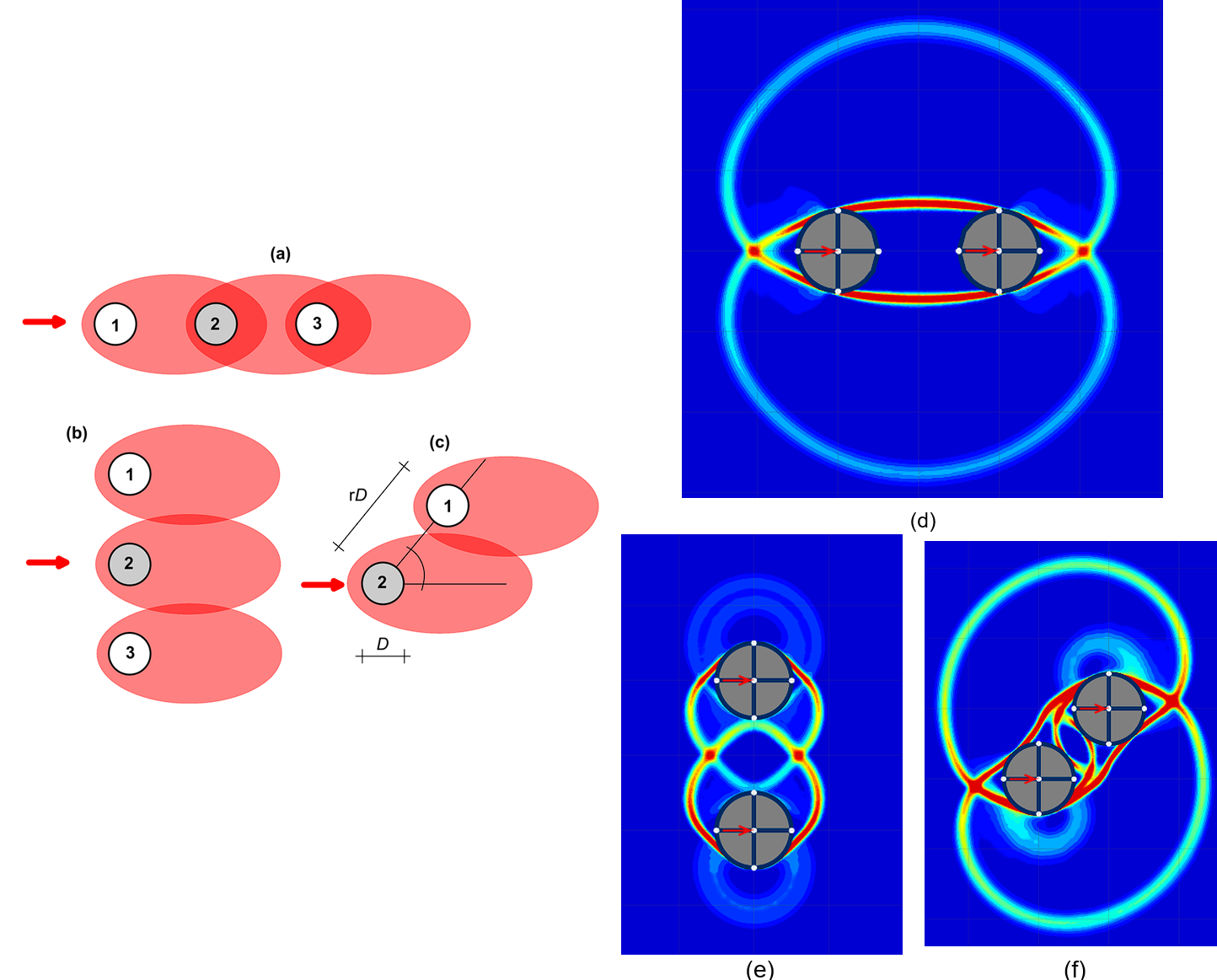
As in the case of pile groups subjected to vertical loads (Chapter 6.20), the response of a group of piles to lateral loadings depends on pile-to-pile interaction effects. More specifically, the lateral deflection of the piles in a group whose head is connected with a rigid pile cap will be the same, when a lateral load is applied on the cap. If the piles are in line (Figures 6.125a and 6.125d) the lateral soil reaction that will develop on pile #2 for given pile cap deflection is less than the lateral reaction that will develop on a single pile under the same deflection, due to the existence of piles #1 and #3 e.g., pile #2 lies in the “shadow zone” of pile #1. Similarly, if the piles are side-by-side (Figures 6.125b and 6.125e) the soil reaction on pile #2 is influenced by the “edge effect”, again due to the existence of nearby piles #1 and #3. In the more general case of skewed piles (Figures 6.125c and 6.125f), these two effects are combined, rendering the assessment of the pile group response more complex.

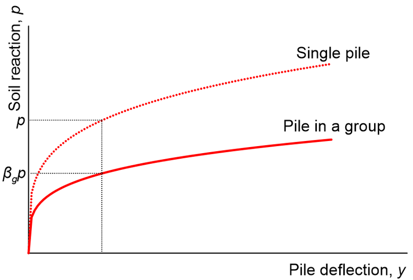
Based on the work of Bogard and Matlock (1983), Brown et al. (1987), and Reese et al. (2006), pile-to-pile interaction effects under lateral loading can be quantified, by multiplying the p-y curve of a single pile (estimated according to Chapter 6.27) with a reduction factor βg (Figure 6.126) that depends on the geometry of the group, the relative position of the pile in the pile group, and the direction of loading.

Figures (a), (b) and (c) on the left present horizontal cross-sections of a three pile group loaded along its strong axis (a) a three pile group loaded along its weak axis (b), two skewed piles loaded horizontally (c). Stresses developing in soil due to pile loading are indicated graphically, and areas of stress overlapping are identified. Figures (d), (e) and (f) on the right present three horizontal cross sections of numerical simulations of a two-pile group subjected to horizontal forces acting along different directions. The complex failure mechanisms that are developing in soil are visualised by means of energy dissipation contours.
Figure 6.125. Influence of pile spacing on pile-soil-pile interaction: (a) Schematic of piles in line; (b) Schematic of piles side-by-side; (c) Schematic of the general case with piles at an angle with respect to the direction of the load; Plane-strain horizontal sections of rigid piles translating laterally in undrained soil: (d) piles in line; (e) piles side-by-side; (f) general case. The energy dissipation contours depict the shape of the composite failure surface mobilised when the ultimate soil reaction is reached.
Graph presenting the p-y curves of a single pile, and of a pile is a group. The p-y curve of the pile is a group results by multiplying p values of the single pile curve by a factor βg that is less than one.
Figure 6.126. Employing the group factor βg to modify p-y curves for pile group effects.

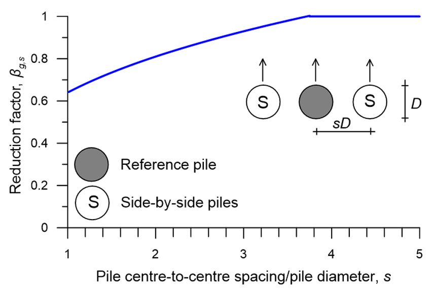
When the direction of the lateral load is perpendicular to the pile row (piles side-by-side), the reduction factor that accounts for interaction of any two side-by-side piles βg,s can be determined on the basis of Figure 6.127, as function of the piles’ centre-to-centre spacing/pile diameter ratio, s :

(6.157) {\beta _{g,s}} = 0.65{s^{0.34}}{\rm{ \:for\: }}1 \le s < 3.75

(6.158) {\beta _{g,s}} = 1{\rm{ \:for\: }}3.75 \le s

All piles in the group must be considered when estimating the reduction factor, as discussed later. In the simple case of three piles spaced at sD depicted in Figure 6.127, the reduction factor that needs to be applied to the py curves of the middle reference pile will be equal to the product of the interaction factors of the reference pile (ref) with each one of the two side-by-side piles (S):

(6.159) \beta _g^{ref} = \beta _{g,s}^{ref \leftrightarrow S} \times \beta _{g,s}^{ref \leftrightarrow S}{\rm{ \:superscripts\:}}{{\rm{ }}^{{\rm{ref}} \leftrightarrow {\rm{S}}}}{\rm{ \:etc}}{\rm{. denote \:interaction \:between \:piles \:ref \:and\: S}}

Chart presenting the variation of the reduction factor βg,s with the ratio of the pile spacing s over the pile diameter D. A schematic of a reference and two side-by-side piles is also shown.
Figure 6.127. Reduction factor βg,s for piles in a row (side-by-side).

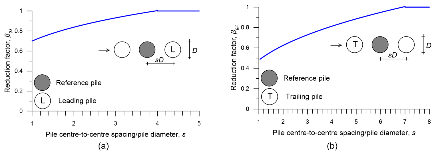
When the direction of the load is parallel to the pile row, the reduction factor for any given reference pile can be determined from Figure 6.128. For quantifying the interaction of the reference pile with the leading pile (L), Figure 6.128a is used to determine the factor βg,l. Similarly, for quantifying the interaction of the reference pile with the trailing pile (T), factor βg,t is determined from Figure 6.128b. The relevant expressions are:

(6.160) {\beta _{g,l}} = 0.7{s^{0.26}}{\rm{\: for\: }}1 \le s < 4.00

(6.161) {\beta _{g,l}} = 1{\rm{ \:for\: }}4.00 \le s

(6.162) {\beta _{g,t}} = 0.48{s^{0.38}}{\rm{ \:for \:}}1 \le s < 7.00

(6.163) {\beta _{g,t}} = 1{\rm{ \:for \:}}7.00 \le s

Figure (a) on the left presents the variation of the reduction factor βg,l with the ratio of the pile spacing s over the pile diameter D. A schematic of a reference and a leading pile is also shown. Figure (b) on the right presents the variation of the reduction factor βg,t with the ratio of the pile spacing s over the pile diameter D. A schematic of a reference and a trailing pile is also shown.
Figure 6.128. Reduction factor (a) βg,l for leading pile in a line (b) βg,t for trailing pile in a line (in-line).

All piles in the group must be taken into account when estimating the reduction factor for each pile. In this simple case of three piles shown in Figure 6.128, the reduction factor of the middle reference (ref) pile will be equal to the product of the factor that accounts for interaction of the reference pile with the leading pile (L), and of the factor that accounts for interaction of the reference pile with the trailing pile (T):

(6.164) \beta _g^{ref} = \beta _{g,l}^{ref \leftrightarrow L} \times \beta _{g,t}^{ref \leftrightarrow T}{\rm{ superscripts}}{{\rm{ }}^{{\rm{ref}} \leftrightarrow {\rm{L}}}}{\rm{ etc}}{\rm{. denote \: interaction \:between \:piles \:ref \:and \:L}}

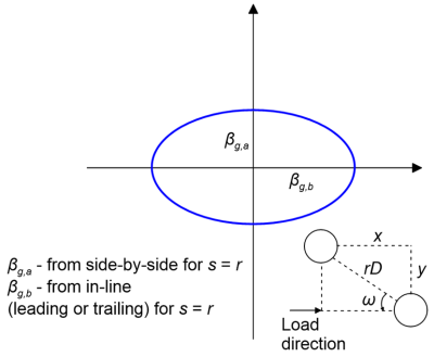
In the general case of two skewed piles (Figure 6.129), the following procedure applies:

  • Determine the factor βg,a from Figure 6.127 for side-by-side piles, while taking into account the distance between the pile centers, rD.
  • Determine the factor βg,b from Figure 6.128 for in-line piles, depending which pile is considered (leading or trailing). Again, take as spacing the distance between the pile centers, rD.

Accordingly, the reduction factor for two skewed piles is estimated by means of geometric considerations as:

(6.165) {\beta _{g,sk}} = \sqrt {{\beta ^2}_{g,b}{{\cos }^2}\omega + {\beta ^2}_{g,\alpha }{{\sin }^2}\omega }

From the above it is clear that the value of the reduction factor depends not only on the arrangement (geometry and spacing) of the piles, but also on the direction of the load.

Diagram illustrating a horizontal cross-section of two skewed piles. The distance between the centre of the two piles along the horizontal direction is x, and the distance between the centre of the two piles along the vertical direction is y. The radial distance of the centres of the two piles is denoted as rD. The angle formed between the line connecting the two pile centres and the load direction is denoted with ω. Two factors are defined. The factor βg,a is obtained from the side-by-side graph for s=r. The factor βg,b is obtained from the in-line (leading or trailing) chart for s=r
Figure 6.129. Estimating the reduction factor βg,sk of skewed piles. Angle ω is defined as the angle between the direction of the load and the line connecting the centers of the piles.

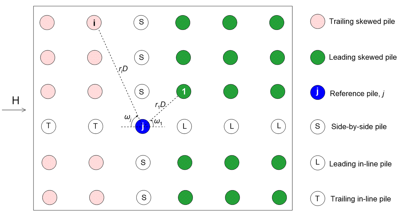
The above can be applied for determining the reduction factor of any individual pile in a multiple pile group. The group reduction factor of pile j in a group comprising n piles may be found by multiplying the reduction factors determined as above, while considering interaction with all the other piles in the group (Figure 6.130).

(6.166) \beta _g^j = \beta _{g,sk}^{j \leftrightarrow 1} \times \beta _g^{j \leftrightarrow 2} \times ... \times \beta _{g,sk}^{j \leftrightarrow i} \times ... \times \beta _g^{j \leftrightarrow n};i \ne j{\rm{ \:superscripts\:}}{{\rm{ }}^{{\rm{j}} \leftrightarrow {\rm{1}}}}{\rm{ etc}}{\rm{. denote \:interaction \:between \:piles \:j \:and \:1}}

Plan view of a pile group consisting of multiple piles. A horizontal force is acting on the pile group. A reference pile is identified as pile j. The remaining piles are classified as trailing skewed pile, leading skewed pile, side-by-side pile, leading in-line pile and trailing in-line pile, depending on the location of the pile in the group relatively to the reference pile and to the direction of the horizontal force.
Figure 6.130. Estimating the reduction factor βgj of a random pile j in a multiple pile group.

This procedure, which must be followed for each individual pile of the group, is demonstrated in the following Example 6.16.

License

Icon for the Creative Commons Attribution 4.0 International License

Fundamentals of foundation engineering and their applications Copyright © 2025 by University of Newcastle & G. Kouretzis is licensed under a Creative Commons Attribution 4.0 International License, except where otherwise noted.