6.19 Immediate settlement of single piles
State-of-practice methods for predicting settlement of single piles (driven piles or drilled shafts) are still very much based on simplified mathematical models of piles and their surrounding soil. Predictions of such models for typical pile/soil parameter combinations are often compiled by authors of relevant publications into “design charts”, to relieve users from the onerous task of programming the rather convoluted expressions. The vast majority of such mathematical models are based on the theory of elasticity, and as such require adopting a series of assumptions, the main of which is that both pile and soil behave as linear elastic, and no separation (slippage) takes place at the soil-pile interface. Comparison of model predictions with measurements obtained during field tests has proven that these assumptions are reasonably accurate under serviceability conditions, when the load acting on the pile head is relatively low, and non-linearity effects can be ignored. Of course today it is relatively straightforward to numerically model a single pile subjected to an axial compressive load (see Examples 6.3 and 6.4), thus obtain direct estimates of settlement without being limited to specific combinations of parameters for which the design charts have been prepared for, while non-linear soil behaviour and slippage at the soil-pile interface can certainly be accounted for even in simple models. This however has not rendered simplified methods obsolete.
It is important to keep in mind that, as settlement is estimated while considering serviceability loads, we may assume that the full serviceability load Qw is transferred through skin friction when the skin friction resistance Qsf is higher than the serviceability load:
(6.90) 
If the serviceability load Qw is higher than the available skin friction resistance Qsf, then we can effectively assume that the load transferred along the pile shaft through friction under serviceability conditions Qsfw is equal to the skin friction resistance Qsf. The remaining of the load Qbw is transferred to the pile toe:
(6.91) 
In other words, the skin friction resistance of the pile is fully mobilised before any load is transferred to its toe.
As the serviceability load is transferred from a pile to the soil predominantly via friction at the soil pile-interface, with little change in the normal stress, the bulk of settlement of a single pile will develop immediately after the load is applied (immediate, or elastic settlement). Consolidation settlement is of the order of 15% of the total settlement for individual piles driven through saturated clay, and generally is not explicitly calculated.
The methods presented in the following for the calculation of immediate settlement of single piles consider compressible piles, hence elastic shortening ρs is inherently considered in the analysis.
6.19.1 Estimation of settlement of compressible friction piles in homogeneous soil
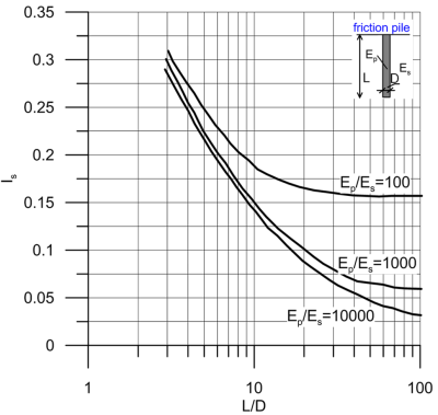
Poulos (1989) describes elasticity-based solutions for predicting settlement of a single cylindrical friction pile embedded in a homogeneous elastic soil layer of infinite thickness. Under these conditions, settlement of a single friction pile ρe (the subscript e refers to elastic settlement, that will develop immediately after application of the load) can be calculated as:
(6.92) 
where Qw is the serviceability load applied at the pile head, D is the diameter of the pile and Es is the Young’s modulus of the soil layer. The factor Is, which actually is the inverse of the dimensionless vertical stiffness of the pile head (vertical stiffness = axial load/vertical settlement Q/ρ), can be estimated from Figure 6.66. It depends on the ratio of the Young’s modulus of the pile Ep over the (drained E′ or undrained Eu depending on the soil type) Young’s modulus of the soil Es. Note that the original solutions by Poulos consider undrained incompressible soil (Poisson’s ratio vs = 0.5) therefore, strictly speaking, Figure 6.66 is applicable only to piles in clay and Es = Eu. However, it is common to use this chart for piles in drained soil too, as the effect of the Poisson’s ratio of soil on pile settlement is not particularly prominent. This is demonstrated later in this Chapter.
Note here that in case the pile is not solid (i.e., is a hollow cylindrical pipe pile), the moduli ratio or relative pile material stiffness Kp = Ep/Es should be calculated as:
(6.93) 
In the special case of a solid pile it is Kp = Ep/Es. In lack of a more accurate (and equally simple) solution, if the soil’s Young modulus is not uniform along the length of the pile, a weighted average can be used together with Eq. 6.92 as (Figure 6.67):
(6.94) 
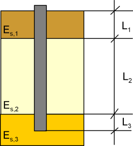
Cases where considering a weighted average soil modulus is reasonable and cases where it can lead to important error in the estimation of settlement are discussed in the following.
6.19.2 Estimation of settlement of compressible friction piles in homogeneous soil of finite thickness
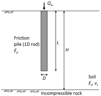
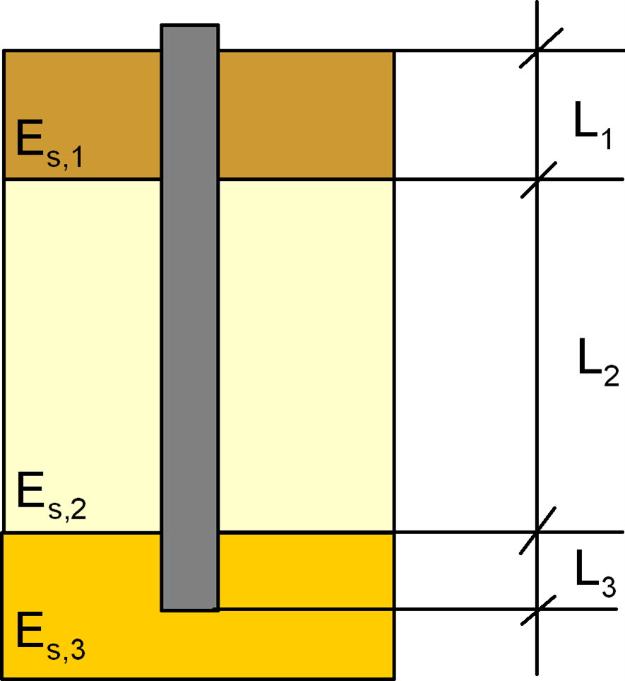
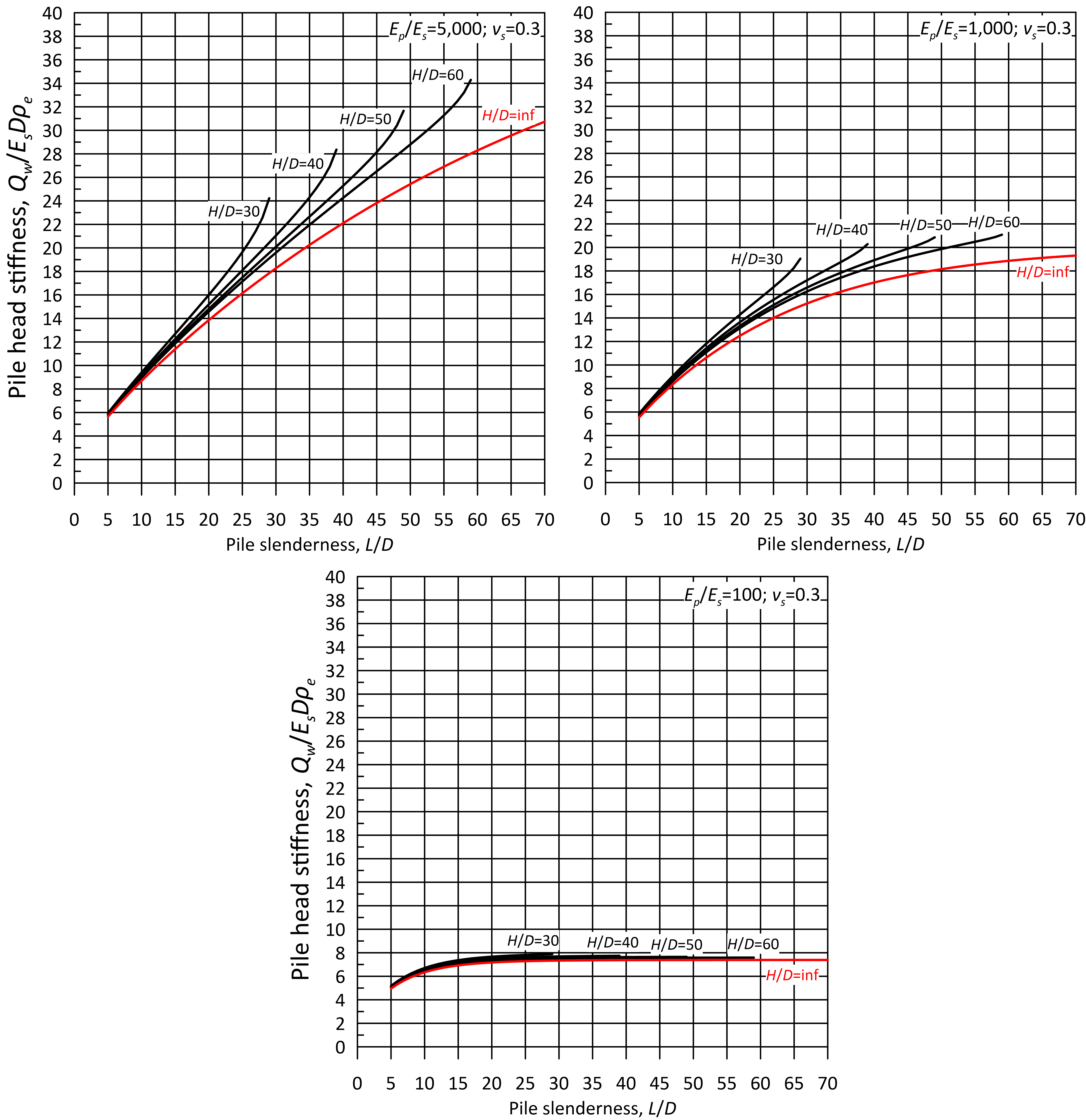
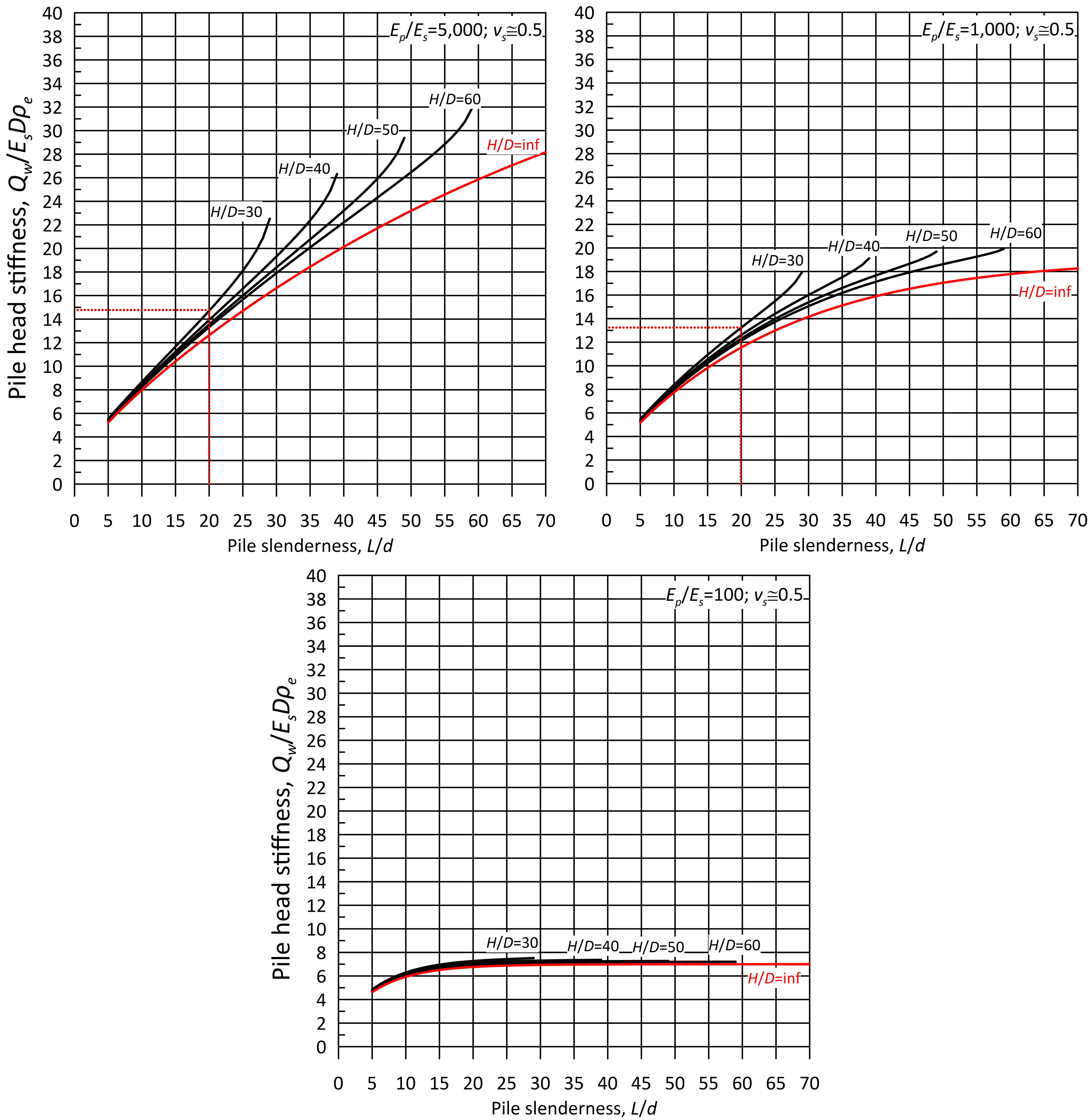
One important drawback of the method presented above is that the thickness of the foundation stratum is assumed infinite. This cannot be the case in practice, thus Poulos’ method will result in overestimating settlement if the bedrock is found at relatively shallow depth. A rigorous elasticity method applicable to cylindrical friction piles embedded in a homogeneous soil layer of finite thickness has been recently proposed by Zheng et al. (2023). A schematic of the problem considered by Zheng et al. is shown in Figure 6.68. The friction pile features diameter D and length L and is embedded in a soil layer of finite thickness H. The method explicitly accounts for the Poisson’s ratio of soil, and is applicable to both drained (e.g., soil Poisson’s ratio vs = 0.3 and soil modulus Es = E′) and undrained conditions (soil Poisson’s ratio vs = 0.5 and soil modulus Es = Eu).
Figures 6.69 and 6.70 provide the dimensionless pile head stiffness Qw/EsDρe as function of the Poisson’s ratio of soil vs, the moduli ratio Ep/Es or Kp for non-solid piles (Eq. 6.93), the pile slenderness L/D and the dimensionless thickness of the soil layer H/D. When H/D = inf Figures 6.69 and 6.70 provide identical results to the Poulos (1989) method. Comparison of Figures 6.69 and 6.70 confirms that the Poisson’s ratio of soil does not significantly affect pile settlement, as stated earlier.


6.19.3 Estimation of settlement of compressible end bearing piles in homogeneous soil
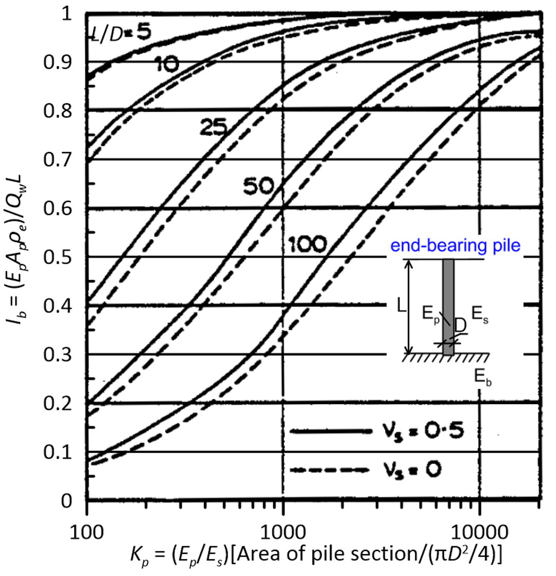
Poulos and Davis (1991) describe a method for calculating settlement of end-bearing compressible cylindrical piles embedded in a uniform elastic soil layer of thickness equal to the pile length L, underlaid by rigid end-bearing stratum (bedrock).
If the end-bearing stratum is much stiffer than the overlying soil layer (Young’s modulus of the bedrock Eb is much larger than the Young’s modulus of the soil layer around the pile shaft Es) then we can use Figure 6.71 to estimate the pile head stiffness factor Ib, and subsequently the elastic settlement of a single end bearing pile ρe for given serviceability load Qw. The curves plotted in Figure 6.71 correspond to the two extreme values of soil Poisson’s ratio vs = 0.5 and vs = 0. Again, the effect of soil Poisson’s ratio on pile settlements is not particularly prominent.
![Graph showing the variation of the factor Ib=(EpAp ρe)/(QwL) with Kp(Ep/Es)[Area of the pile section)/(πD^2/4)]. Ten curves for different L/D values and Poisson's ratio values vs = 0.5 and vs = 0 are shown. The characteristics of an end bearing pile are shown in an inset figure: The length of the pile is denoted with L, its diameter is denoted with D, the Young's modulus of the pile's material is denoted with Ep, the Young's modulus of soil is denoted with Es and the Young's modulus of the end bearing stratum is denoted with Eb.](https://oercollective.caul.edu.au/app/uploads/sites/143/2025/03/6.71-hr-e1743553940528.png)
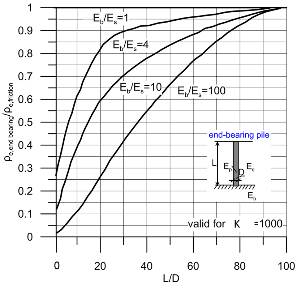
The compressibility of the bedrock will have an effect on the predicted settlement of end-bearing piles, particularly for short piles (low L/D values) when significant portion of the serviceability load will actually be transferred to the pile toe. Figure 6.72 below presents the effect that the stiffness of the bedrock has on end bearing pile settlement. To compute the settlement of an end bearing pile on the basis on Figure 6.72, we assume first that the total load is transferred through shaft friction, and estimate the pile settlement ρe,friction as:

(6.95) 
where Is is read from Figure 6.66. Then, using Figure 6.72, we can estimate the settlement of the end bearing pile, as a function of the pile slenderness (L/D) and the ratio of the Young’s modulus of the end bearing layer Eb over the Young’s modulus of the overlying soil layer(s) Es. Figure 6.72 presents results for typical relative pile stiffness Kp = 1000.
Notice in Figure 6.72 that the settlement of slender piles (L/D > 50) is not influenced significantly by the compressibility of the bearing stratum. In other words, if we seek to reduce the settlement of a relatively long pile, it is preferable to increase its diameter or stiffness, rather than increasing its length to found its toe on a deep, stiff layer.
6.19.4 Estimation of settlement of compressible end bearing piles in layered soil
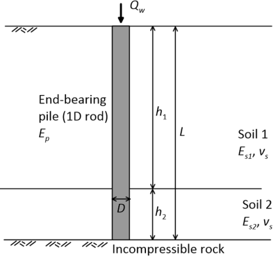
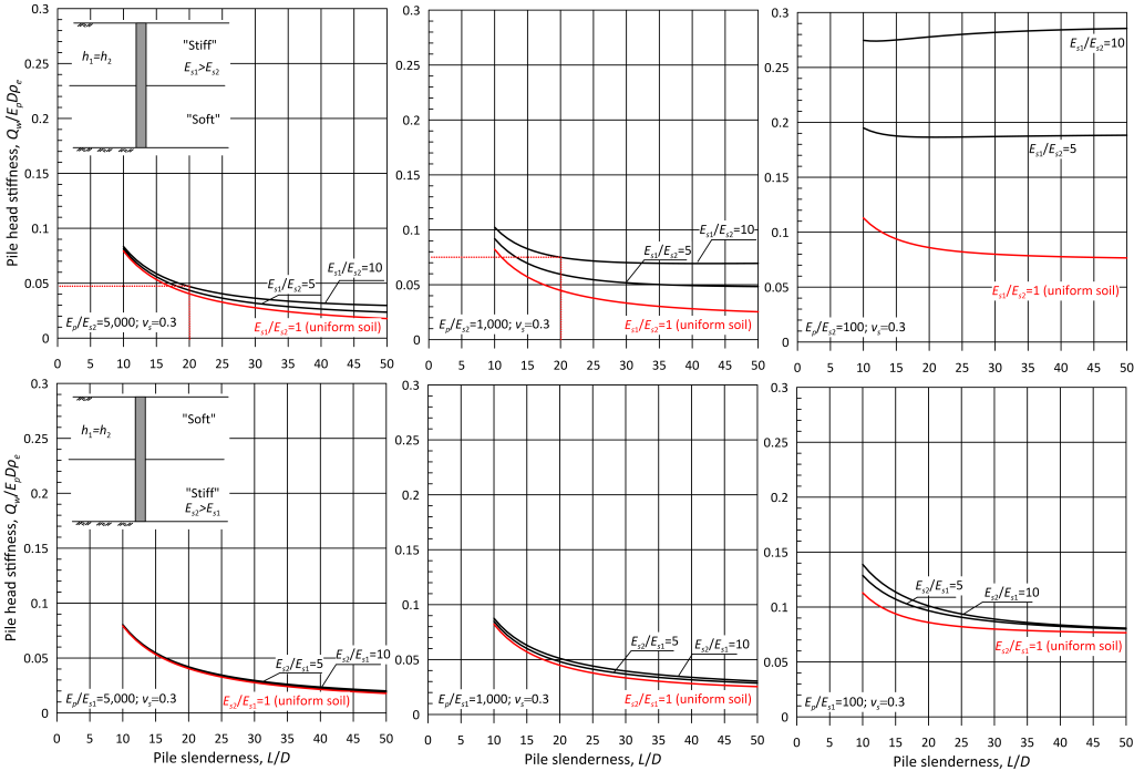
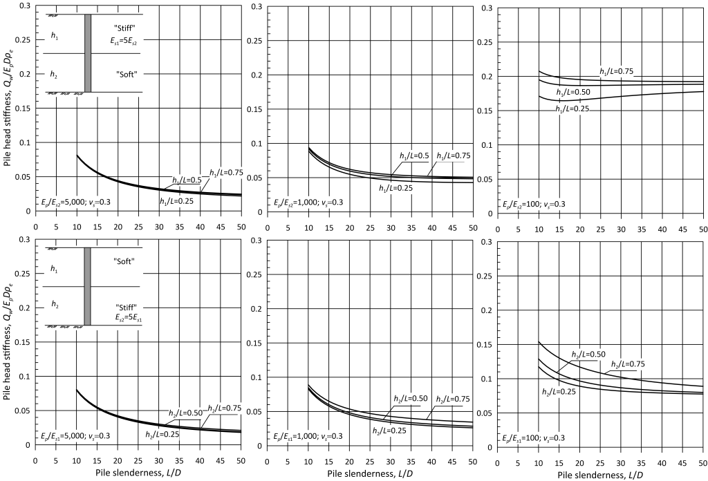
It has been discussed earlier that estimating settlement of a pile in layered soil with methods developed for uniform soil conditions along the pile shaft may lead to inaccurate predictions, even when a weighted average soil modulus in considered in the analysis. This problem has been tackled by Zheng et al. (2024), who developed an elasticity method for predicting settlement of end bearing piles resting on rigid bedrock (Eb = infinite) driven through soil that consists of two soil layers that feature different properties. The problem they considered is depicted in Figure 6.73.
Zheng et al. produced charts that provide the dimensionless pile head stiffness Qw/EpDρe as function of the modulus of the pile Ep, the moduli of the soil layers Es1 and Es2, pile slenderness L/D, and the thickness of the soil layers h1 and h2. These charts are presented in Figures 6.74 and 6.75, and can be used to directly estimate settlement of end-bearing piles for any serviceability load Qw. The results presented in the mentioned figures demonstrate that the role of top layer to pile head stiffness (thus pile settlement) is more important than the role of the bottom layer. Thus, using a weighted average soil modulus (Eq. 6.94) together with homogeneous soil models may lead to inaccurate settlement predictions when the surficial soil layer is stiffer than the underlying soft soil. On the other hand, considering a weighted average soil modulus may be a reasonable approximation if soil stiffness increases with depth, for example for piles in sand.
