6.13 Design of drilled shafts socketed in soft rock to resist axial compressive loads
Methods developed for the design of piles founded in soil are not appropriate (i.e., will probably result in particularly conservative designs) if used to design drilled shafts which toe is socketed into even relatively soft rock, such as the sandstone/siltstone formations encountered along the East Coast of Australia. As such, design of drilled shafts socketed in soft rock in practice is performed using custom methods, such as the method of Rowe and Armitage (1987a), which has been used successfully for the design of numerous projects in Australia. Rowe and Armitage’s method is based on satisfying a design settlement criterion when the drilled shaft is subjected to a factored axial compressive load at its head, and ensuring that collapse (bearing capacity failure) under the same axial load will be avoided. Therefore, there is no clear differentiation between Serviceability Limit State (SLS) and Ultimate Limit State (ULS), as the method had originally been developed to be used together with traditional partial safety factors (limit state design). Here the method is adapted to conform with AS2159 requirements. Note that the following are applicable to rockmass without significant presence of weak seams. If this is the case, the reader is referred to the original publications of Rowe and Armitage for the expressions required to adjust the method. However, the general concepts described in the following remain the same.
It should be noted that the method of Rowe and Armitage, and the associated “design charts” presented in the following, have resulted from numerical analyses of a single pile subjected to an axial compressive load. Hence, instead of using the provided charts etc., one can attempt to replicate Rowe and Armitage simulations, and design the drilled shaft on the basis of project-specific numerical simulations. For the model to be able to successfully simulate the behaviour of socketed drilled shafts, it is critical that the shear resistance at the shaft-rock interface is modelled properly, and the parameters recommended in Rowe are Armitage have been validated against numerous tests on sandstone/siltstone formations. Rowe and Armitage have used an elastic-perfectly plastic failure criterion for the interface, and account for degradation of interface strength with increasing relative displacement, as well as (degrading) dilation angle to account for interface roughness. Details on the model are provided in Rowe and Armitage (1987b).
6.13.1 Design of a fully socketed drilled shaft
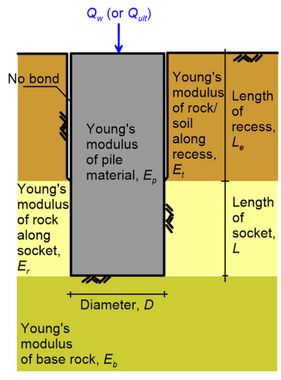
If the drilled shaft is not recessed i.e., the interface between the shaft and the rock is fully bonded (Length Le = 0, Figure 6.30) and there are no weathered seams along the wall of the socket, the design method is as follows:
Step 1:
We first determine the design parameters. These include an initial estimate of the pile diameter D, the design settlement ρD, which depends on the requirements of the project, the modulus of the drilled shaft Ep, which depends on concrete properties, and the characteristic value of the unconfined compressive strength of rock cores σc, from the interpretation of unconfined compressive (UCS) tests on rock samples. Point Load test results can be used to supplement UCS test data, however the Geotechnical Engineer must appreciate the uncertainties associated with using point load test data to estimate the unconfined compressive strength, and factor these uncertainties in the selection of the characteristic σc value. In addition, the design axial compressive load at the ULS (Qult = S*) and the serviceability axial compressive load (Qw) acting on the pile head must be estimated, using AS1170 provisions and appropriate load factors for Qult. Note that usually the settlement criterion will govern the design, and not the ULS collapse load criterion. Since SLS axial compressive loads calculated according to AS1170 are not factored, the maximum acceptable settlement value must be prudently selected, to account for the probability of exceedance of the predicted settlement through the design life of the project.
Step 2:
Estimate the characteristic value of the side shear resistance that can develop at the shaft-rock interface τd and the characteristic values of the rockmass Young’s modulus Eb underneath the shaft toe and along the length of the socket Er. Note that the symbol τd is used here to denote side shear resistance developing on piles in rock, instead of the symbol fsf used in the previous sections to denote skin friction resistance of piles in soil, despite both being shear stresses at the interface between a pile and its surrounding medium. In lack of site-specific data, the following expressions by Rowe and Armitage (1984) can be used to estimate the abovementioned parameters from the characteristic value of the unconfined compressive strength of rock cores σc (in MPa).
(6.58)  for regular clean sockets (roughness R1-R3: Table 6.7)
(6.59)  for clean rough sockets (roughness R4: Table 6.7)
(6.60) 
Step 3:
Calculate the dimensionless socket length L/D required for the entire serviceability load to be carried by side shear:
(6.61) 
| Roughness class | Description |
|---|---|
| R1 | Straight, smooth-sided socket, grooves or indentations less than 1 mm deep |
| R2 | Grooves of depth 1 to 4 mm, width greater than 2 mm, at spacing 50 to 200 mm |
| R3 | Grooves of depths 4 to 10 mm, width greater than 5 mm, at spacing 50 to 200 mm |
| R4 | Grooves or undulations of depth greater than 10 mm, width greater than 10 mm, at spacing 50 to 200 mm |
The subscript max in the above Eq. 6.61 denotes the dimensionless socket length required for all the load to be carried by side shear i.e., no load is to be transferred to the shaft’s toe.
Step 4:
Calculate the design settlement influence factor Id:
(6.62) 
Step 5a:
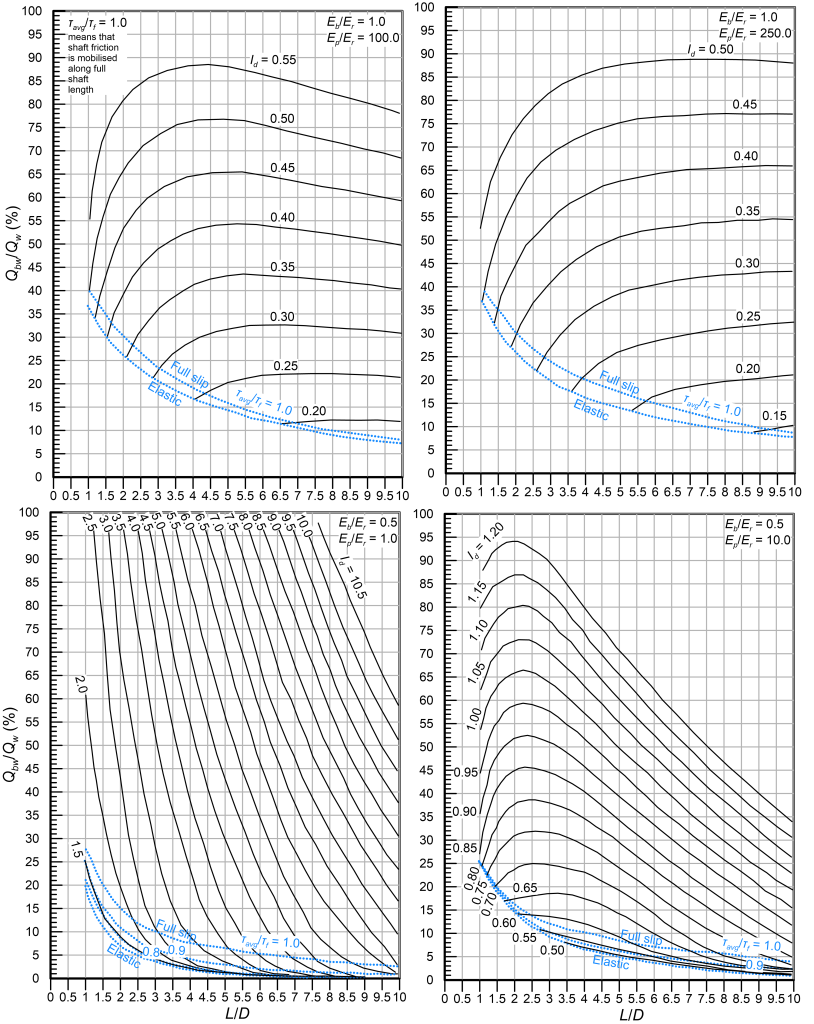
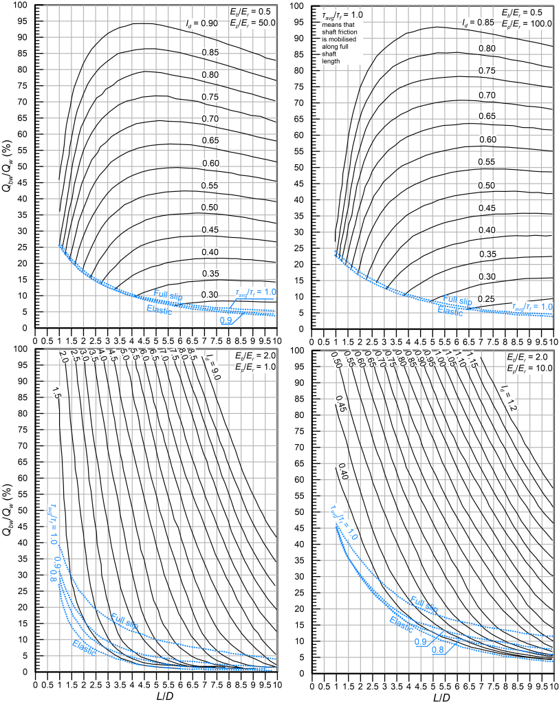
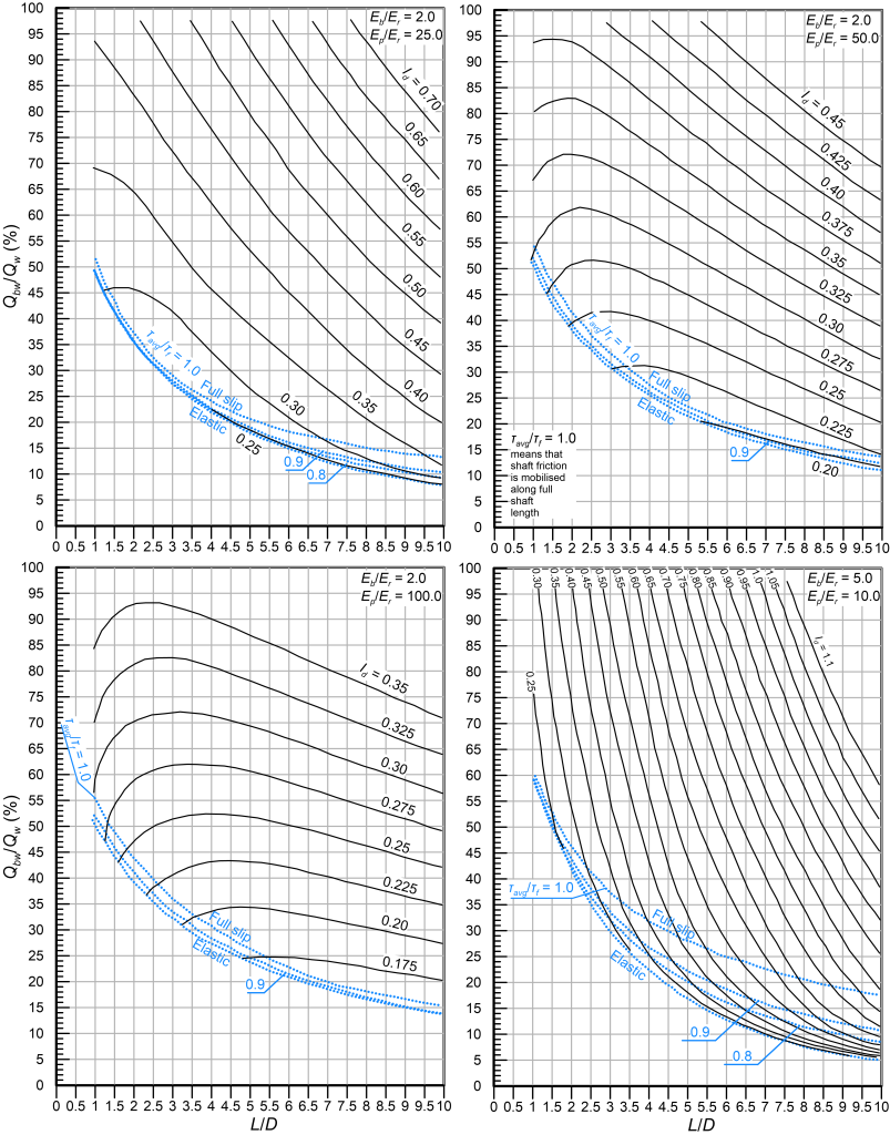
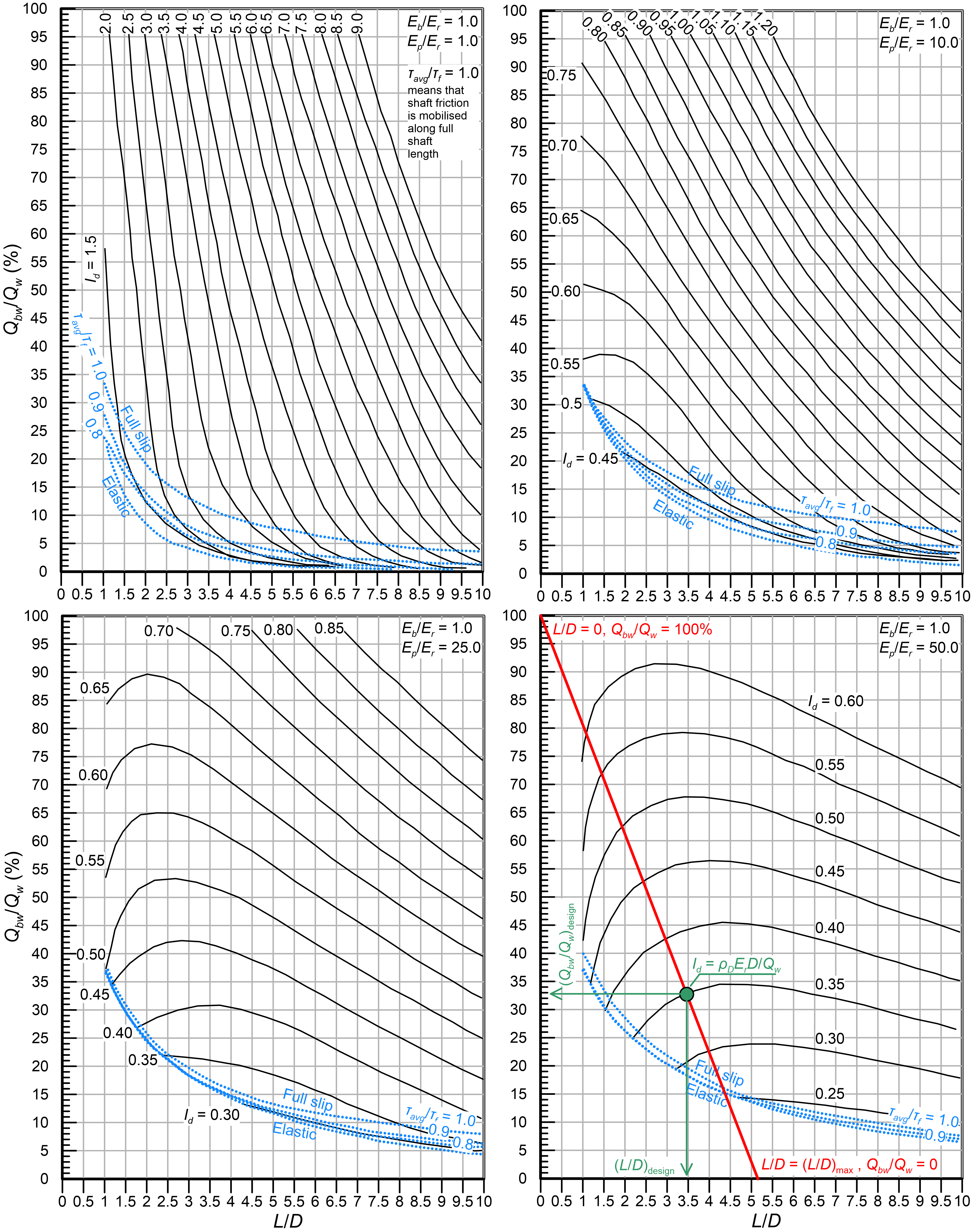
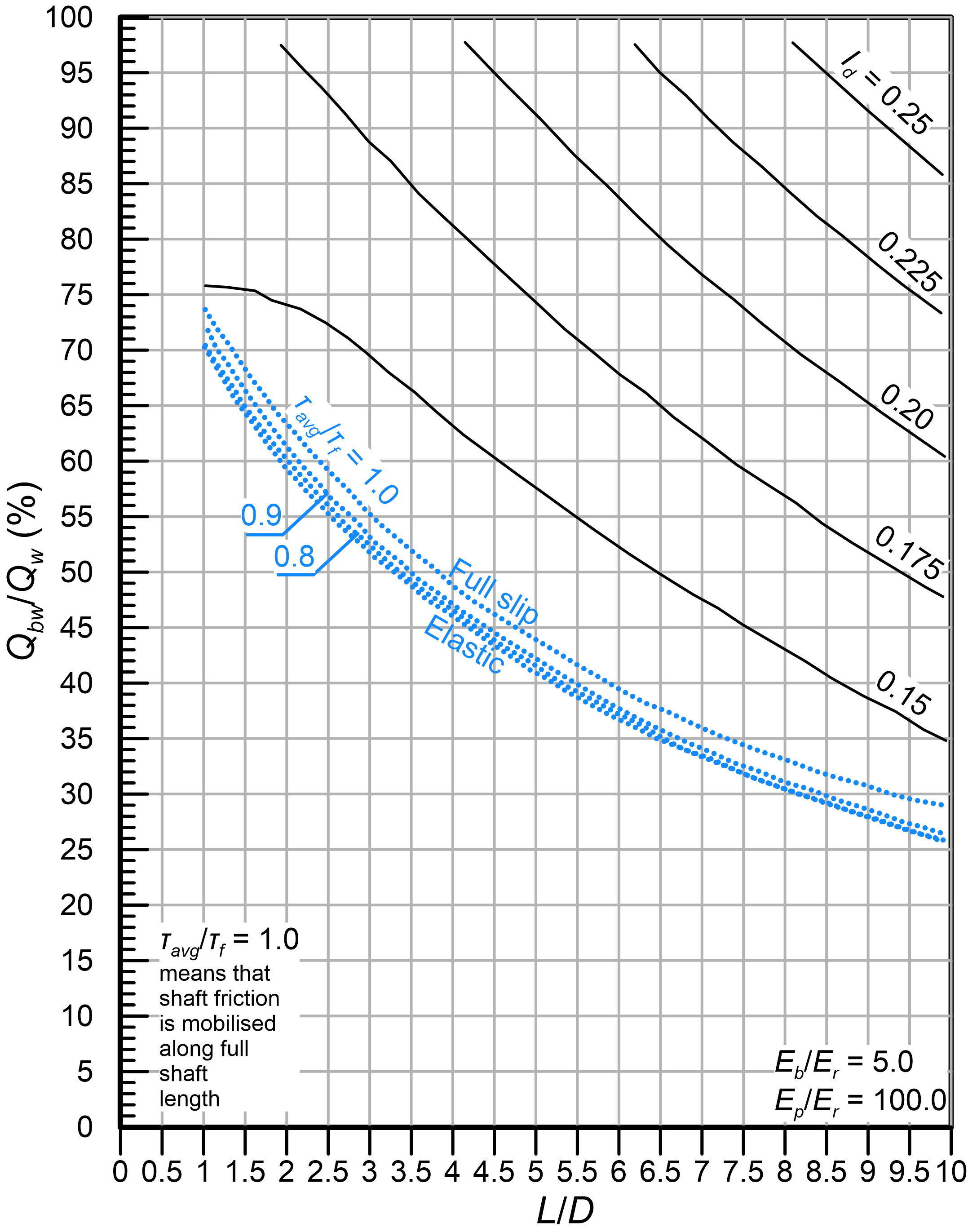
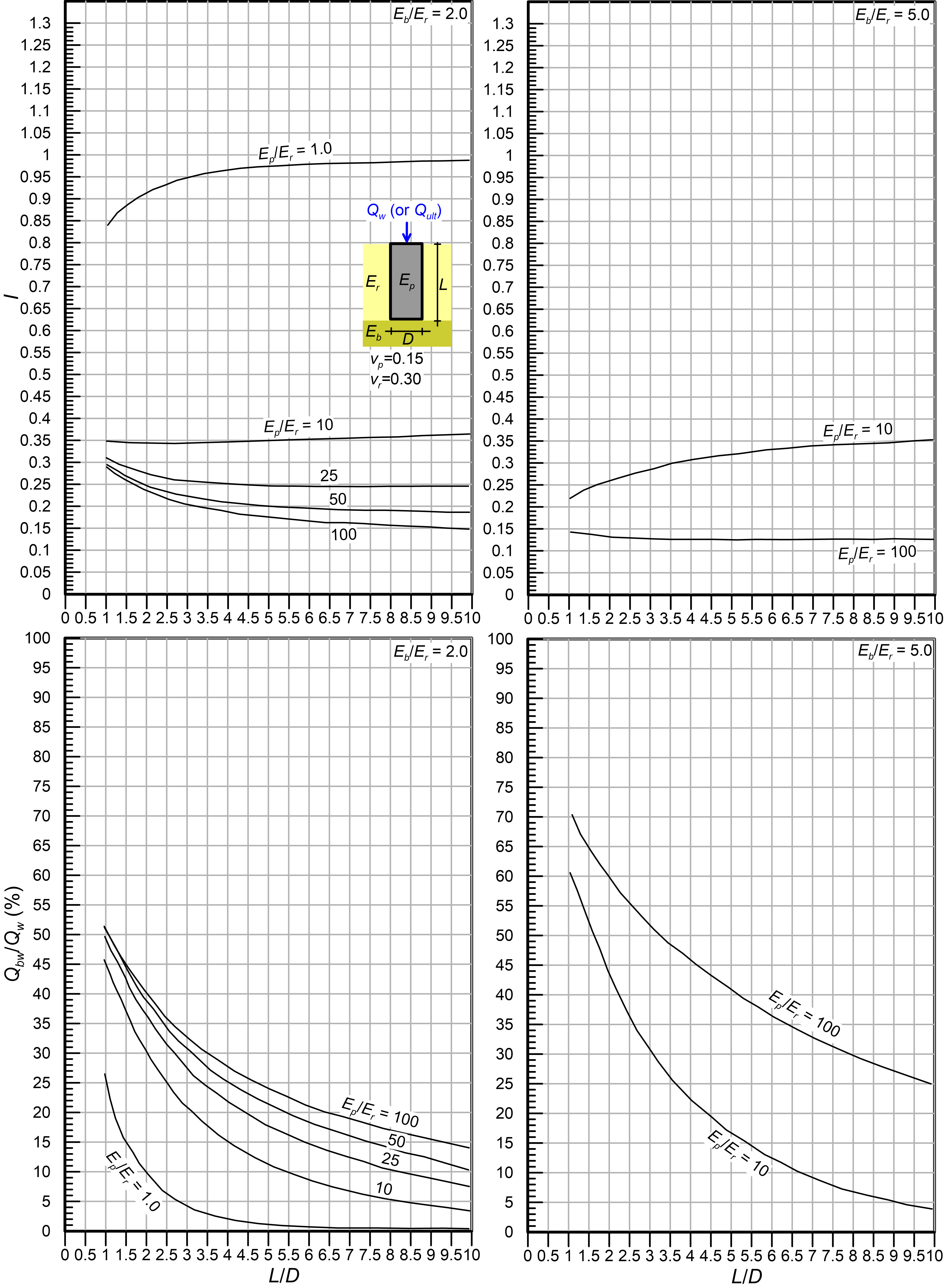
We can now select the length of the socket L (see Figure 6.30) required to achieve the target design settlement influence factor, while allowing for slip at the shaft-rock interface i.e., a percentage of the serviceability load Qw transferred to the toe of the shaft. This requires calculating first the dimensionless moduli Ep/Er and Eb/Er and selecting the appropriate design chart from Figures 6.31 to 6.35. Accordingly, we draw a straight line that connects the coordinates (L/D = 0, Qbw/Qw = 100%) and (L/D = (L/D)max, Qbw/Qw = 0) i.e., the red line drawn indicatively in Figure 6.31. Here Qbw is the serviceability load transferred to the toe of the shaft, expressed as a percentage of the serviceability load applied at the head Qw. The intersection of that straight line with the curve corresponding to the Id value calculated from Eq. 6.62 provides: i) The design dimensionless length (L/D)design, from which the required pile length to satisfy the settlement criterion is calculated, and ii) The design load ratio (Qbw/Qw)design that provides the load transferred to the toe of the shaft under serviceability conditions.
Step 5b:
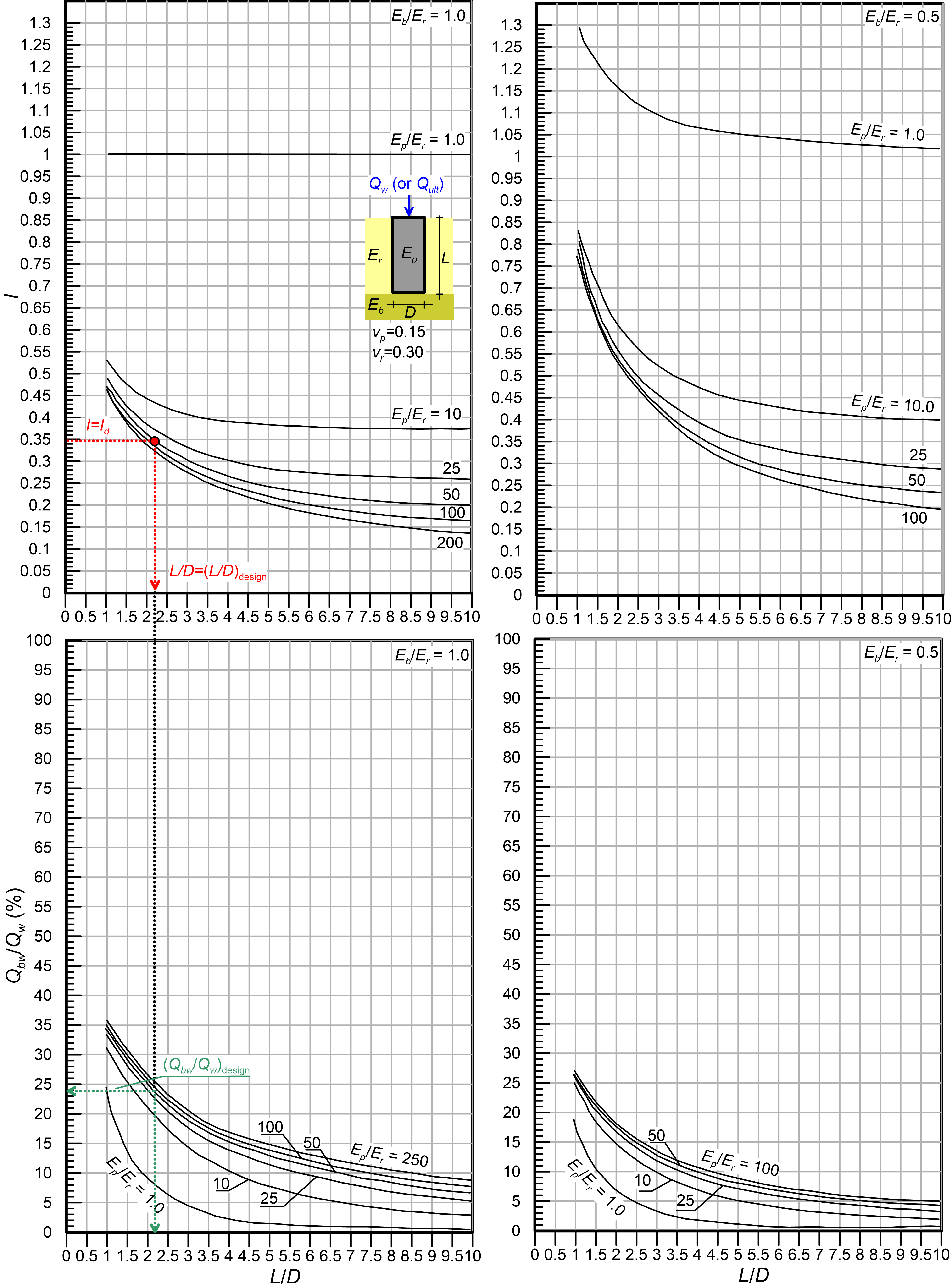
It is not guaranteed that an intersection of the straight line connecting (L/D = 0, Qbw/Qw = 100%) and (L/D = (L/D)max, Qbw/Qw = 0) and of the curve corresponding to the Id value calculated from Eq. 6.62 can be found. In this case we need to check first if the drilled shaft can be designed so that no slip occurs at the shaft-rock interface under serviceability conditions (elastic design). This is achieved by selecting first the appropriate chart from Figures 6.36 and 6.37 and drawing a horizontal line on the elastic settlement factor I charts for I = Id i.e., the red line drawn indicatively in Figure 6.36. If this line intersects the Ep/Er curve corresponding to the particular shaft, the drilled shaft can be designed elastically, and the required dimensionless pile length (L/D)design can be read from the same figure (see Figure 6.36). Next, the percentage of the serviceability load transferred to the toe (Qbw/Qw)design can be estimated from the elastic load distribution charts, as presented indicatively in Figure 6.36.
Step 5c:
If no intersection point can be found between the horizontal line I = Id and the Ep/Er curve, then the pile must be re-designed, by changing the selected diameter D (or the settlement criterion).
Step 6:
Following the design of the pile to satisfy the serviceability criterion, we must now check that the pressure at the toe of the shaft does not exceed the allowable value at the ultimate limit state. The end bearing stress at the toe of the shaft is calculated as:
(6.63) 
An important assumption underlying the above Eq. 6.63 is that the percentage of the load transferred at the toe remains the same under both SLS and ULS conditions. This may not be the case e.g., if the pile has been designed elastically for serviceability conditions. As such we should calculate the load ratio (Qb/Q)design under ULS conditions by repeating Steps 3-5 while considering Qult instead of Qw in the denominator and an appropriate settlement value e.g., ρ=(Qult/Qw)ρD. The axial stress at the toe of the shaft must be lower than the unconfined compressive strength of rock, multiplied by the geotechnical reduction factor:
(6.64) 
The above criterion intends to ensure that no significant yielding will take place in the rock underneath the shaft toe. In addition to that, the end-bearing resistance at the base of the shaft qbf must not exceed 2.5 times the factored unconfined compressive strength φgbσc:
(6.65) 
The factor 2.5 in Eq. 6.65 resulted from field tests on socketed piles, and is the base pressure when yield of the drilled shaft was observed as a change in the shape of the load-displacement curve. The limiting end-bearing pressure qbf is calculated as:
(6.66a) 
(6.66b) 
The factor f in Eq. 6.66 intends to ensure that even when the rock-shaft friction mobilised in the field is less than the value assumed in the design τd, there will be sufficient margin of safety against collapse. Rowe and Armitage recommend to take f = 0.3 i.e., to assume that only 30% of the expected shear resistance is mobilised. Both Eqs 6.64 and 6.65 must be satisfied for the design to be acceptable.
6.13.2 Design of a recessed drilled shaft
Rowe and Armitage recommend to initially completely ignore the contribution of the surficial layers (length Le where no bond exists at the shaft-rock interface, Figure 6.30) to the axial capacity of recessed drilled shafts, and design the shaft according to the steps 1-6 above. This approach will produce a reasonably accurate design if the drilled shaft is designed so that slip at the socketed shaft length-rock interface takes place i.e., if an intersection point can be established in the charts presented in Figures 6.31 to 6.35. Elastic shortening of recessed piles may contribute significantly to their settlement. Therefore, the elastic shortening of the recess, calculated using theory of elasticity while considering the recessed section of the pile as 1-D rod as ρs = 4LeQw/(πD2Ep), must be subtracted from ρD when calculating the design settlement influence factor for recessed piles, Id in Step 4.
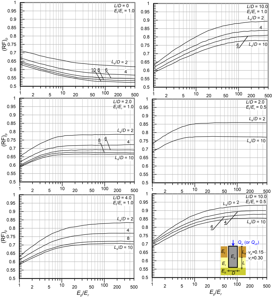
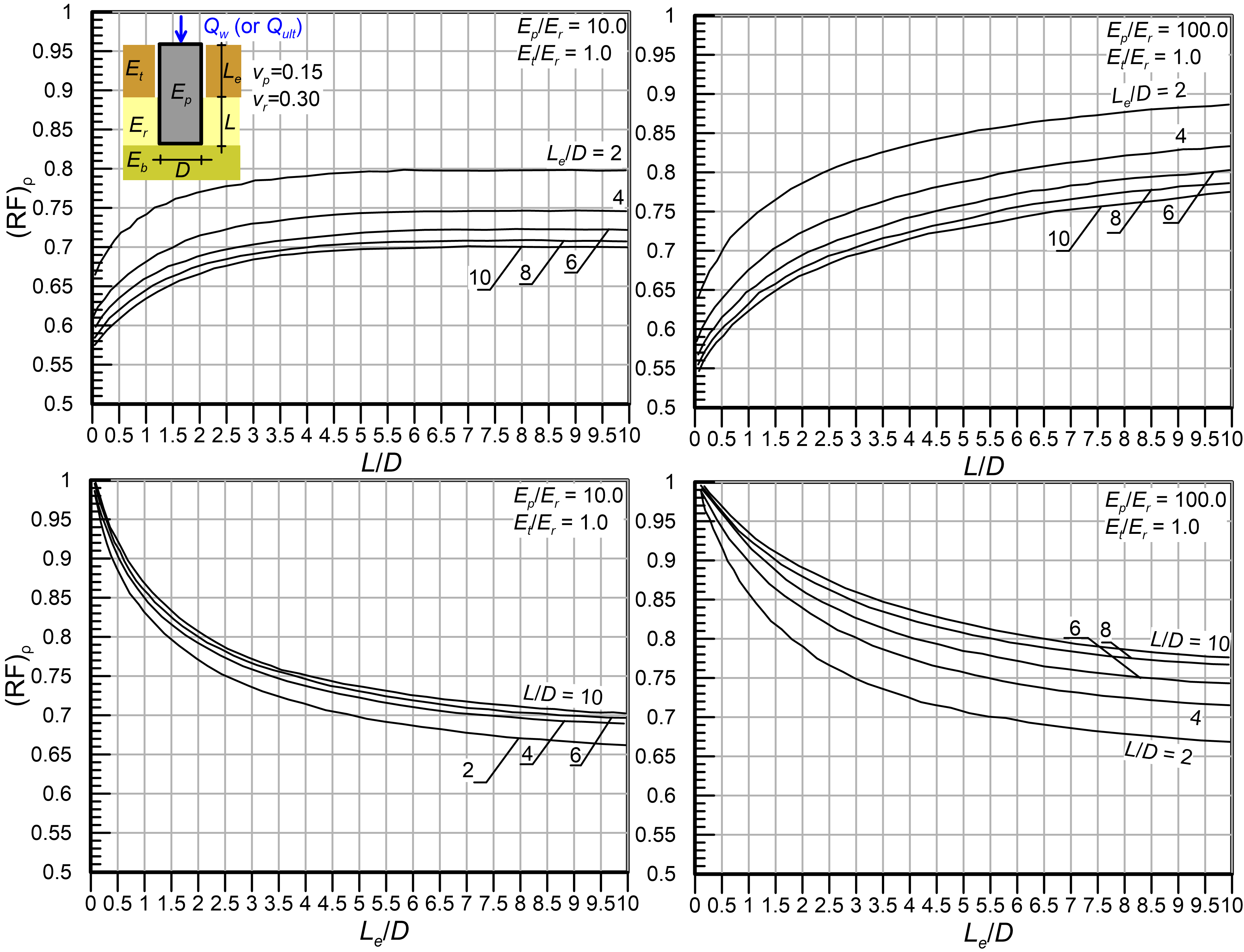
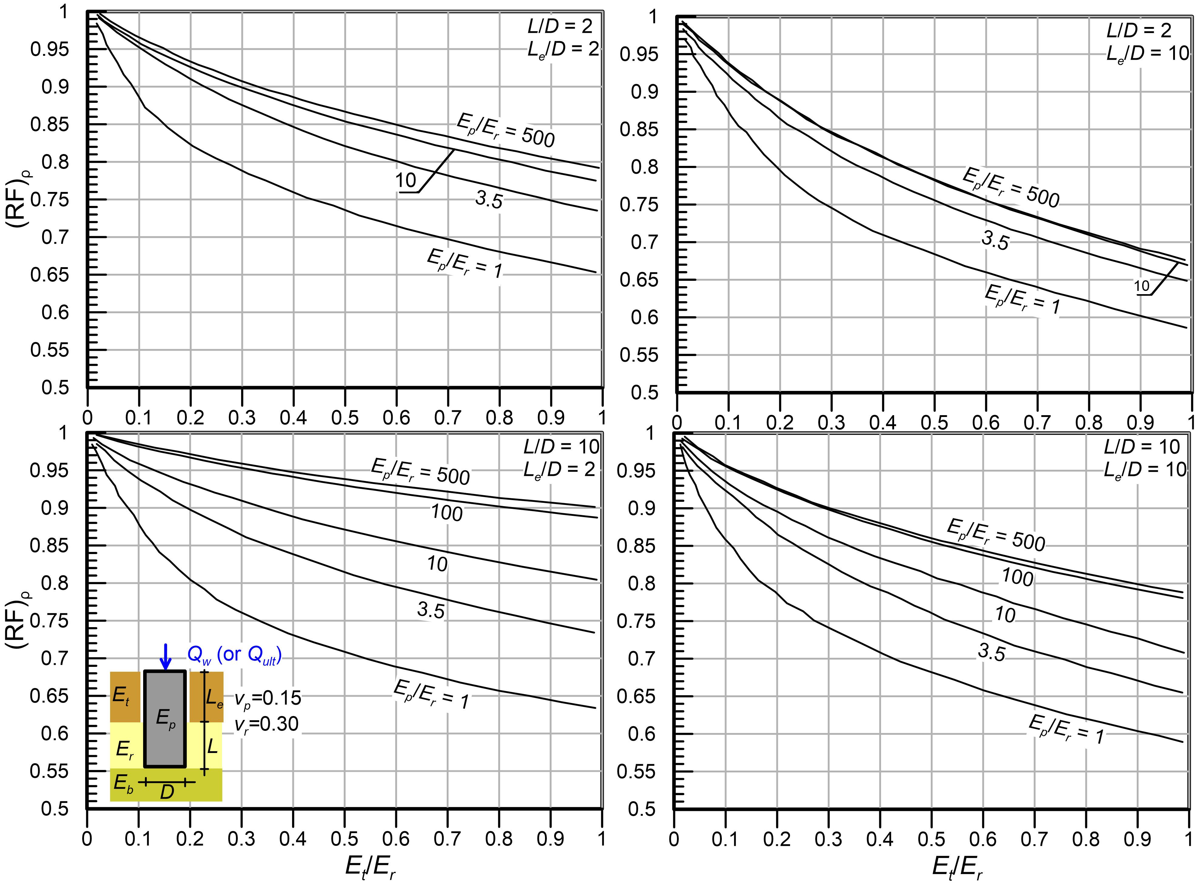
However, if an intersection point could not be established, and the shaft is designed to perform elastically following step 5c, ignoring the contribution of the surficial layers may be too conservative. In this case, the contribution of the recessed part of the drilled shaft to the axial capacity can be accounted for in the design as follows: After having calculated the design dimensionless length (L/D)design from step 5a, calculate the settlement reduction factor (RF)ρ from Figures 6.38 to 6.40 as function of the parameters L/D, Le/D, Et/Er and Ep/Er (see Figure 6.30 for definitions). Subsequently adjust the design settlement influence factor Id as:
(6.67) 
and repeat step 5b using the adjusted value of the settlement influence factor I*d. During repeating step 5c a new value of (L/D)*design will be calculated, therefore (RF)ρ may have to be calculated again and the process may have to be iterated until convergence is achieved.
Notice from Figure 6.40 that if the recess consists of (relatively soft) soil layers i.e., the ratio of Et/Er attains values significantly lower than unity, then the settlement reduction factor (RF)ρ attains values close to unity i.e., the contribution of shaft resistance along the part of the pile in soil to reducing settlement of the drilled shaft will be trivial.


