5.6 Numerical modelling of footings resting on the surface of drained soil
The numerical analysis results presented in Example 5.5 demonstrate that the use of equivalent strength parameters together with an associative flow rule provides reasonable estimates of the bearing capacity of foundations, while avoiding numerical instabilities that stem from using as input the actual friction angle and dilation angle of drained materials, and consequently of non-associative flow rule.
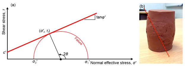
However, this is not the only potential source of numerical instabilities in simulations where we seek to estimate the bearing capacity of shallow foundations. Unlike undrained soils modelled with the Mohr-Coulomb Undrained material model, where shear strength does not depend on stress levels, drained soils modelled with the Mohr-Coulomb Drained material model will feature zero shear strength near the model surface if i) Their effective cohesion is set to be zero (see Figure 5.4), and ii) The footing is not embedded as it is in Example 5.5. Finite element codes have difficulty handling materials of zero strength, and the simulation may end prematurely (before the bearing capacity is reached) due to poor convergence. While using as input a nominal effective cohesion c′ ≈ 1 kPa to avoid modelling a material of zero strength near the surface where geostatic stresses are zero will certainly improve numerical stability, this is not always sufficient.
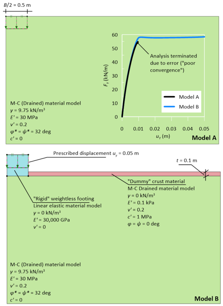
An alternative modelling strategy is illustrated in Figure 5.49: Instead of applying a prescribed displacement directly on the model surface (Model A) to obtain the force-displacement curve, as we did e.g., in Example 5.2, we apply the prescribed displacement on the top of a geometry cluster representing the footing (Model B). A weightless linear elastic material of very high stiffness is assigned to that cluster, to model a rigid footing. On the model surface we introduce a weightless thin crust, as another separate geometry cluster. To this cluster we assign a material of arbitrarily high cohesion (“infinite” strength) but also of very low stiffness, so that the stresses that will develop in this “dummy” crust will be extremely low, and will not contribute to a fictitious increase in the predicted bearing capacity. Notice that we still use Davis equivalent parameters φ*, ψ* for the actual soil, but we have considered its effective cohesion c′ to be zero.
Results of the two model variants are presented in Figure 5.49, in terms of the predicted force-displacement curve. Observe that Model A failed to reach the collapse load, and the analysis ended prematurely with an error message. That is despite the fact that arc-length control was used to solve the system of non-linear equations, which can provide solution to problems where softening is expected, i.e., when the stiffness matrix is not always a positive definite through the analysis. On the other hand, Model B’s analysis was completed successfully, and the collapse load can be inferred from the force-displacement curve. Notice also that, up to the analysis stage where Model A’s analysis failed, both models produced identical results. This suggests that the introduced technique facilitates convergence, at no expense of model accuracy.
