5.3 Some fundamentals of the bearing capacity of shallow foundations
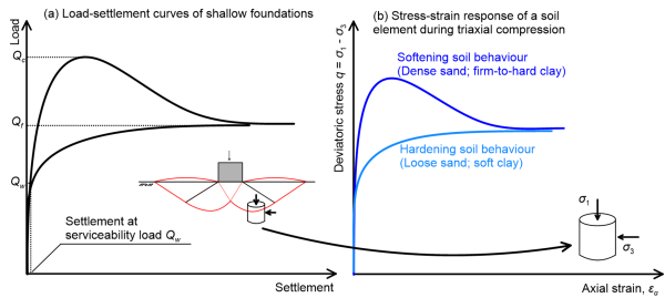
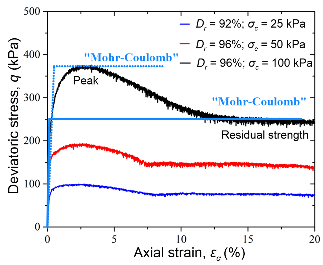
With the term bearing capacity of a foundation we have defined the maximum pressure that the foundation can safely carry. For dilating soils that exhibit softening behavior (see Figure 5.5) failure corresponds to the peak shear stress, while for non-dilating (contractive) soils that exhibit hardening behavior, failure corresponds to the critical state shear stress, where shearing takes place under constant volume conditions. Sometimes, the term failure load is used to refer to the ultimate geotechnical strength in terms of force for contractive soils, and the term collapse load is used for dilating soils (Figure 5.21). Here we prefer to use the term collapse load Qf to describe the ultimate geotechnical strength in terms of force for both dilating and contractive soils, as we use the Mohr-Coulomb failure criterion to quantify soil strength, and we do not differentiate between peak and residual strength (Figure 5.5). Keep in mind that the settlement associated with the design capacity may not be acceptable. Thus, apart from:
(5.8) 
serviceability requirements must be taken into account for the proper design of a foundation.
It is reminded here that settlement calculations are always performed with specific serviceability load combinations, in accordance with AS1170.0 and AS1170.1 for structures other than bridges, and in AS5100.2 for bridges. The geotechnical reduction factor φg does not apply when calculating settlement with the characteristic values of soil compressibility parameters, according also to AS5100.3.
Let’s consider now the simplified case of a rigid strip footing resting on elastic-perfectly plastic soil (Figure 5.22). As the footing begins to settle upon load application, it “traps” a wedge of soil, which pushes its way downwards. According to our assumptions, initially the soil will respond elastically. It will be compressed vertically and extend laterally. Energy from the acting load is stored into the soil, as elastic energy.
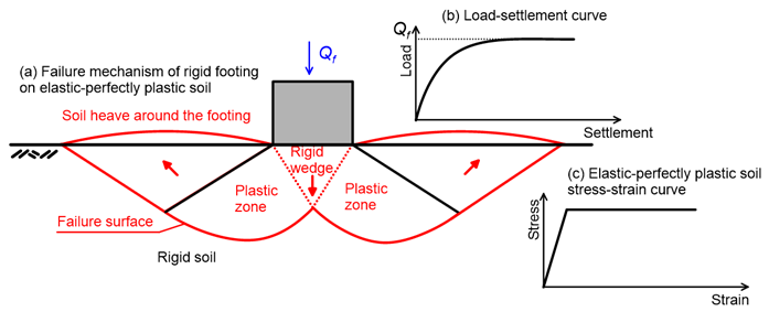
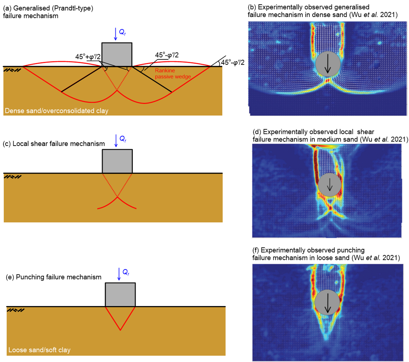
As the load increases, some regions of the soil will yield, forming plastic zones. Upon further increase of the load, plastic zones evolve to the ground surface around the footing, and appear with the form of heave (Figure 5.22a). There is an intermediate zone between elastic and perfectly plastic behavior, where the soil behaves as elasto-plastic material, and deformation is essentially only lateral. In reality, soil heave around the footing is influenced by the overburden pressure, and the strain-hardening ability of the material. If the footing is embedded into the soil and/or the material has a large potential to strain-harden, soil heave will be restrained and large lateral pressures will develop. In that case, a strain-softening material would behave as a strain-hardening material (we have mentioned earlier that dilatancy depends on the level of confining stress) pushing the plastic zone further into the soil mass, and the general failure mechanism depicted in Figures 5.23a and 5.23b may not fully develop (see Figures 5.23c-f).

Strictly speaking, for the estimation of the bearing capacity of a shallow footing we need to find a solution that satisfies the four general principles:
- Equilibrium.
- Stress-strain relations and failure criteria (e.g., the Mohr-Coulomb failure criterion described above).
- Compatibility of deformations.
- Stress and displacement boundary conditions.
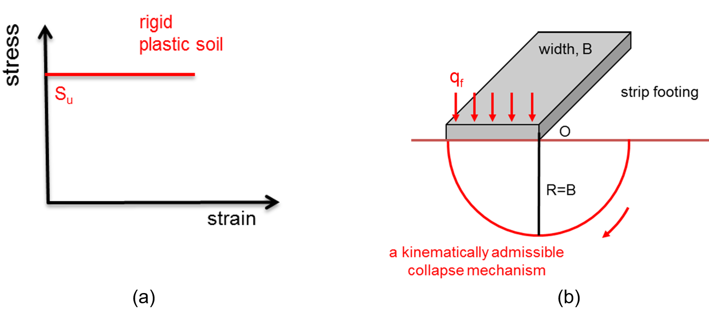
It is not always possible to find a closed-form analytical solution that satisfies all the above. Instead, we can employ the limit theorems of plasticity to calculate upper and lower bound estimates of the bearing capacity. To use these theorems we assume that soil is rigid-plastic i.e., there is no elastic zone and deformations up to failure are zero (Figure 5.24a). Besides, we are not interested in calculating settlement at failure, which according to the definition of bearing capacity can be infinite. In some cases, the upper and lower bounds to the bearing capacity are the same, thus the calculated collapse load is the exact solution. The limit theorems are (Craig and Knappet 2012):
Lower bound theorem: If a state of stress can be found for which the failure criterion in not violated anywhere within the soil, and this state of stress is in equilibrium with the externally applied pressure and internal soil stresses (geostatic stresses), then collapse cannot occur. The externally applied pressure is a lower bound estimate of the exact bearing capacity, as a more efficient stress distribution may exist, which may be in equilibrium with an external pressure of larger magnitude.
Upper bound theorem: Assume a kinematically admissible failure mechanism (that is a failure surface that is continuous and compatible with the boundary conditions). If during a displacement increment along this failure mechanism the work done by external pressures is equal to the dissipation of energy by the soil internal stresses (due to shearing), then collapse must occur. This system of external pressures is an upper bound estimate of the exact bearing capacity, as a more efficient mechanism may exist, that dissipates less energy, which might lead to failure under lower external pressures.
Let’s see how these can be applied for the calculation of the bearing capacity of shallow foundations, by using the upper bound theorem to calculate an upper bound estimate of the bearing capacity qf in terms of stress of a strip weightless footing resting on the surface of semi-infinite, homogenous, isotropic, weightless undrained soil (Figure 5.24b).

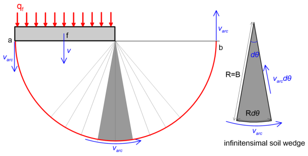
One possible and kinematically admissible failure mechanism comprises a circular arc of radius R equal to the width of the footing B, which center coincides with the edge of the footing. The work done by the pressure applied on the footing is equal to the force qfB multiplied by the relative velocity v during a displacement increment (Figure 5.25), therefore:
(5.9) 
The energy dissipated due to shearing Eshear between the circular failure surface and the stationary soil is equal to the total shear resistance along the slip surface (undrained shear strength x length) multiplied by the relative velocity varc, therefore:
(5.10) 
Where θ for the particular geometry is θ = π. Note that the relative velocity around the edge of the circular arc is constant, and equal to varc = v, as the soil rotates relatively to O. However, we are not done yet with the calculation of internal energy, as we need to add the energy dissipated within the circular arc Eint, due to shearing occurring between soil wedges (Figure 5.25). The length of each wedge is equal to the radius R and the relative velocity is equal to varcdθ (so that the relatively velocity along the radius tends to zero as the wedge becomes infinitesimally small). Therefore, the internal energy dissipated due to shearing between wedges is:
(5.11) 
And the total dissipated energy is:
(5.12) 
If we equate this to the work of the external pressure (Eq. 5.9), we calculate the bearing capacity in terms of stress as:
(5.13) 
The same result can be obtained by means of the limit equilibrium method. In that case we take moments about Point O in Figure 5.24. Moments due to normal forces acting on the arc about O are zero, since their line of action passes through O, therefore any shearing that takes place between wedges does not contribute to the moment equilibrium equation, which becomes:
(5.14) 
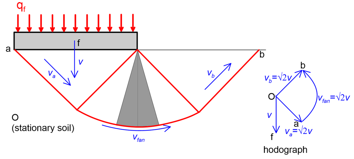
and since R = B it is again qf = 2πSu. Of course, as mentioned earlier, this is an upper bound to the exact bearing capacity. A more efficient mechanism (dissipating less energy) that is still kinematically admissible is the one shown in Figure 5.26, consisting of two rigid blocks a and b and an arc (or shear fan, as it is commonly called) of radius R=B/√2. The bearing capacity corresponding to this mechanism can be found similarly to the arc mechanism described above.

The work done by the external forces is the same as in Eq. 5.9. The energy dissipated due to sliding of the rigid blocks relatively to the stationary soil, as well as sliding of the shear fan relatively to the stationary soil and shearing between its soil wedges is calculated in Table 5.3 below.
| Failure line | Length of failure line | Relative velocity | Energy Eshear due to sliding relatively to stationary soil | Energy Eint due to shearing between soil wedges |
|---|---|---|---|---|
| a |  |
 |
 |
0 (rigid) |
| Fan (θ = π/2) |  |
|
 |
 |
| b | |
|
|
0 (rigid) |
| Total: |  |
|||
Equating the total dissipated energy from Table 5.3 with the work done by the pressure acting on the footing yields the bearing capacity qf = (π+2)Su. This is equal to the exact bearing capacity for a strip footing without surface surcharge, because in this particular case we can find a lower bound solution equal to the upper bound solution. These calculations are omitted as they are beyond the scope of this Part. It should be further clarified here that the mechanism of failure below a strip footing subjected to a vertical pressure will be symmetric, as shown in Figure 5.27.
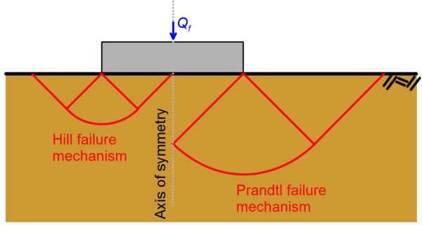
Application of limit analysis theorems suggests that two mechanisms are theoretically possible: the Hill mechanism where horizontal sliding takes place at the soil-footing interface (see also Figure 5.27), and the Prandtl mechanism which is valid also for rough footings, where no sliding takes place. Interestingly, both result in the same bearing capacity, suggesting that the bearing capacity of a strip footing on undrained homogeneous soil is independent of the properties of the soil-footing interface (unlike the case of a circular footing). In reality however, as the undrained strength increases with depth, the bearing capacity of a rough footing will be higher of that of a smooth footing, as the Prandtl-type mechanism mobilises a deeper soil mass, and the mobilised undrained strength will be higher.
The same concept can be employed for determining the bearing capacity of shallow footings under drained conditions, on weightless soil which strength is quantified via the effective parameters cohesion c′ and friction angle φ′ (Effective Stress Analysis). Note that to apply the upper and lower bound theorems, soil must obey an associative flow rule (ψ = φ′). A consequence of that is that correct application of these expressions requires entering the equivalent parameters c*, φ* (Eqs. 5.5-5.7), instead of the actual measured soil parameters. However, this notion is not further explored here, and instead conservative characteristic shear strength parameters are used in the examples, as often done in practice. In addition, since soil is assumed to obey the linear Mohr-Coulomb failure criterion, the friction angle φ′ is independent of stress level.
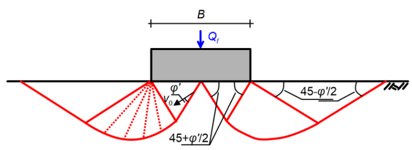
Equating the rate of external work and internally dissipated energy for half of the Hill mechanism shown in Figure 5.28a (as above) yields (Chen 2012):
(5.15) ![\dfrac{1}{2}{Q_f}2{v_0}\cos \left( {\dfrac{\pi }{4} + \dfrac{{\varphi '}}{2}} \right) = c'\left( {{v_0}\cos \varphi '} \right)\left[ {\dfrac{B}{{2\cos \left( {\dfrac{\pi }{4} + \dfrac{{\varphi '}}{2}} \right)}}} \right] + c'\left( {{v_0}{e^{\tfrac{\pi }{2}\tan \varphi '}}\cos \varphi '} \right)\left[ {\dfrac{{B{e^{\tfrac{\pi }{2}\tan \varphi '}}}}{{2\cos \left( {\dfrac{\pi }{4} + \dfrac{{\varphi '}}{2}} \right)}}} \right] + \dfrac{{c'B\left( {{v_0}\cot \varphi '} \right)}}{{2\cos \left( {\dfrac{\pi }{4} + \dfrac{{\varphi '}}{2}} \right)}}\left( {{e^{\pi \tan \varphi '}} - 1} \right)](https://oercollective.caul.edu.au/app/uploads/quicklatex/quicklatex.com-33ab8d71b93709e9908501a0531aa8a2_l3.png "Rendered by QuickLaTeX.com")
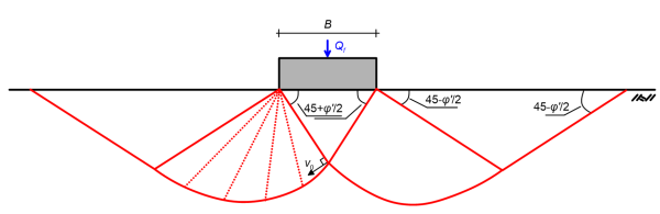
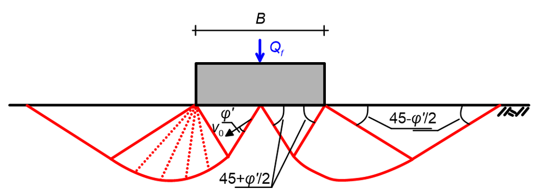
where Qf is the collapse load and v0 is the velocity of the rigid wedge below the footing. Similarly, for the Prandtl mechanism shown in Figure 5.28b (Chen 2012):
(5.16) ![\dfrac{1}{2}{Q_f}{v_0}\cos \left( {\dfrac{\pi }{4} + \dfrac{{\varphi '}}{2}} \right) = c'\left( {{v_0}\cos \varphi '} \right)\left[ {\dfrac{B}{{4\cos \left( {\dfrac{\pi }{4} + \dfrac{{\varphi '}}{2}} \right)}}} \right] + c'\left( {{v_0}\cos \varphi {e^{\tfrac{\pi }{2}\tan \varphi '}}} \right)\left[ {\dfrac{{B{e^{\tfrac{\pi }{2}\tan \varphi '}}}}{{4\cos \left( {\dfrac{\pi }{4} + \dfrac{{\varphi '}}{2}} \right)}}} \right] + \dfrac{{c'B\left( {{v_0}\cot \varphi '} \right)}}{{4\cos \left( {\dfrac{\pi }{4} + \dfrac{{\varphi '}}{2}} \right)}}\left( {{e^{\pi \tan \varphi '}} - 1} \right)](https://oercollective.caul.edu.au/app/uploads/quicklatex/quicklatex.com-f7f9499e049667a34f5f5fd08096acee_l3.png "Rendered by QuickLaTeX.com")
Essentially, Eqs. 5.15 and 5.16 are the same. Notice that the geometry of both mechanisms depends on the friction angle of soil φ′, and degenerates to the geometry shown in Figures 5.26 and 5.27 under undrained conditions, when φu = 0°. In that case the logarithmic spirals forming the shear fans degenerate to circular arcs. Eqs 5.15 and 5.16 can be written in a simpler form while including the effect of the overburden stress qs = γDf for footings embedded at a depth Df as:
(5.17) 
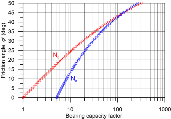
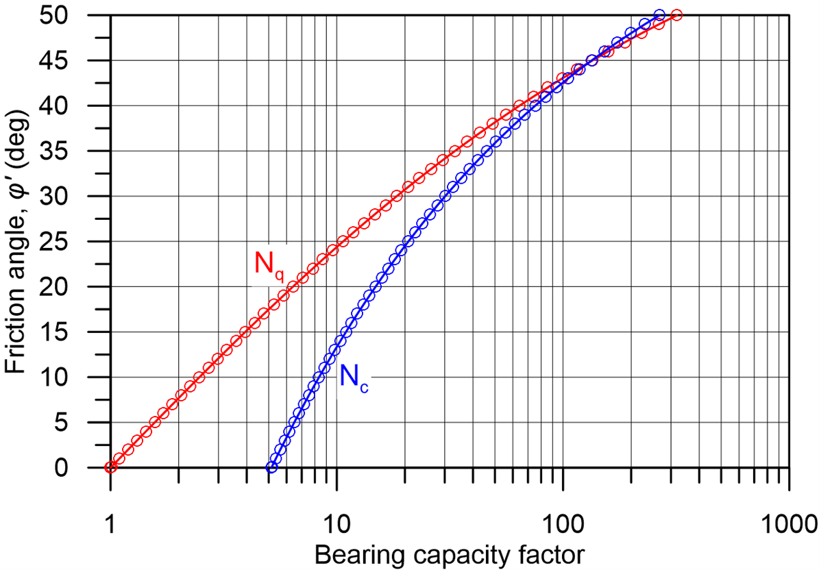
where Nc, Nq are the bearing capacity factors provided from the Eqs. 5.18 and 5.19 and plotted in Figure 5.29 below. Note that the limit of Nc as φ tends to zero (or φu) is equal to Ncu = (2+π), so in that case Eq. 5.17 provides the same collapse load for undrained weightless soil found earlier, since Nq also tends asymptotically to zero as friction angle approaches zero.
(5.18) 
(5.19) 
It is clear from the above expressions that the bearing capacity depends on whether soil response upon loading will be drained or undrained i.e., whether excess pore water pressures will develop. The following Table 5.4 summarises the type of expected soil behaviour as function of the soil grain size distribution and the scope of the analysis (long- or short-term). This table applies mainly to common, static loads. It is reminded that even sands, of high permeability, may develop excess pore pressures and behave as undrained if the rate of loading is sufficiently fast (e.g., during an earthquake).
A consequence of assuming a linear soil failure criterion, thus friction angle independent of confining stress levels, is that the bearing capacity factors Nq and Nγ are independent of the size of the foundation. Despite this not being true, and scale effects (i.e., the negative correlation of bearing capacity factors thus qf in Eq. 5.17 to the dimensions of the foundation) on bearing capacity being documented in the literature, these are customarily ignored for common footing sizes encountered in practice.
| Soil type | Analysis scope | Type of behaviour | Strength parameters |
|---|---|---|---|
| Sand (coarse-grained) or dry soils in general | Long-term or Short-term (no excess pore pressures due to high soil permeability and/or relatively slow loading rate) | Drained | c′, φ′ (ESA) |
| Saturated clay (fine-grained) | Long-term (after dissipation of excess pore pressures) | Drained | c′, φ′ (ESA) |
| Short-term (during or immediately after construction; dynamic loads such as wind/wave action) | Undrained | Su (TSA) | |
| ESA: Effective Stress Analysis |
|||
| TSA: Total Stress Analysis |
|||
