4.7 Immediate and consolidation deformations underneath shallow foundations imposing 3-D loading conditions
A theory of elasticity approach
There are many practical situations where we do not merely seek to predict settlement at the centre of a footing (or a loaded area in general), but instead we wish to predict how a footing or an embankment will deform immediately after construction, and at the end of consolidation e.g., when differential settlement, tilt or even horizontal ground movements are important. This task can be performed analytically by means of theory of elasticity formulas. However, these come with some pitfalls. These pitfalls are explored with the aid of the following example, where predictions of analytical formulas are compared against results of numerical simulations.
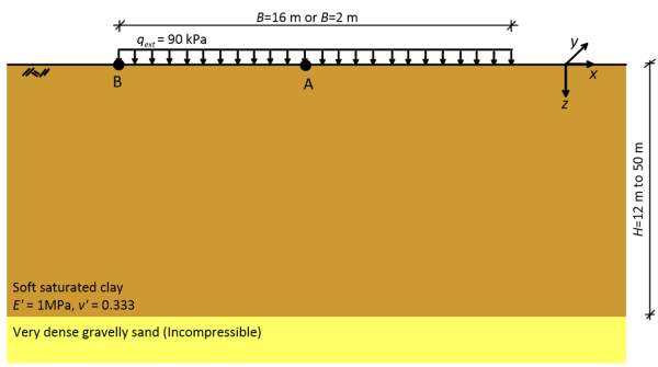
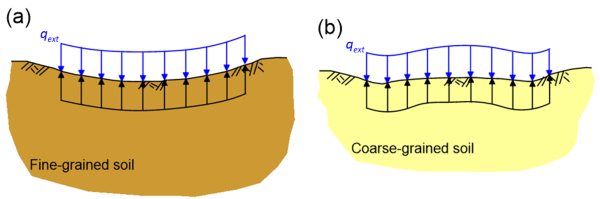
Consider the flexible strip footing applying uniform pressure studied in Example 4.3. The footing is transferring pressure qext = 90 kPa to a soft saturated clay layer, which is underlaid by practically incompressible dense gravelly sand deposits (Figure 4.34). Unlike Example 4.3, here the width of the loaded area B is less than (3 to 4)H, where H is the thickness of the compressible layer. As such we cannot treat this problem as 1-D. Settlement under the centre of the footing will not be equal to settlement near its edges, and the shape of the deformed soil surface will be concave upward, as shown in Figure 4.11. Here we will compute the profile of vertical soil deformations with depth immediately after application of the pressure, and at the end of consolidation at: i) The middle of the footing (Point A, Figure 4.34), and ii) its edge (Point B, Figure 4.34). We will use analytical formulas to compute soil stress and deformations on the basis of theory of elasticity, and we will compare our results to those of PLAXIS simulations. We will not consider geostatic stresses and hydrostatic pore pressures in the calculations, as settlement of elastic materials depends only on the additional stresses applied in soil from the external loading. Finally, the calculations shown below are for uniform soil, however the method is applicable to layered soil too.
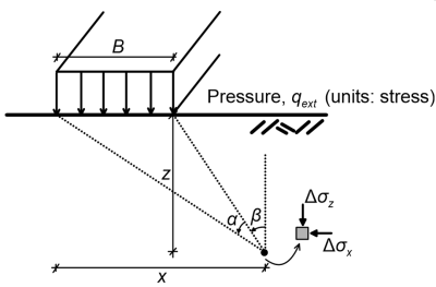
To obtain the profile of deformations at the two selected locations, we must first calculate stress increments with depth due to the strip pressure applied on the surface. Since this problem is plane-strain, out-of-plane-strains and deformations are zero, thus considering the coordinate system of Figure 4.34:
(4.40) 
The remaining expressions for increments of total stress due to a strip pressure acting on the surface of an infinite half-space are provided in Chapter 3.4 and are repeated here for completeness:
(4.41) ![\Delta {\sigma _z} = \dfrac{{{q_{ext}}}}{\pi }\left[ {\alpha + \sin \alpha \cos \left( {\alpha + 2\beta } \right)} \right]](https://oercollective.caul.edu.au/app/uploads/quicklatex/quicklatex.com-ecb79ba9fcbfc4f335a02d055b2b6ead_l3.png "Rendered by QuickLaTeX.com")
(4.42) ![\Delta {\sigma _x} = \dfrac{{{q_{ext}}}}{\pi }\left[ {\alpha - \sin \alpha \cos \left( {\alpha + 2\beta } \right)} \right]](https://oercollective.caul.edu.au/app/uploads/quicklatex/quicklatex.com-a858d8bcf3ee10ed76843754a33fd781_l3.png "Rendered by QuickLaTeX.com")
(4.43) 
(4.44) ![\Delta {\tau _{zx}} = \dfrac{{{q_{ext}}}}{\pi }\left[ {\sin \alpha \sin \left( {\alpha + 2\beta } \right)} \right]](https://oercollective.caul.edu.au/app/uploads/quicklatex/quicklatex.com-48e31b9b994d856324d1beabd0be54d1_l3.png "Rendered by QuickLaTeX.com")
where, referring to Figure 3.7, α = 2atan[(B/2)/z] and β = -atan[(B/2)/z] at Point A, while α = atan[(B/2)/z] and β = 0 at point B; v′ is the drained Poisson’s ratio of soil. Notice that we have three normal stress components here, which generally are all non-zero. Hence the problem is described as three-dimensional. Although these are not used as input in the calculation of soil vertical deformations, the expressions that provide principal stress increments under plane-strain conditions are shown below, for completeness.
(4.45) ![\Delta {\sigma _1} = \dfrac{{{q_{ext}}}}{\pi }\left[ {\alpha + \sin \alpha } \right]](https://oercollective.caul.edu.au/app/uploads/quicklatex/quicklatex.com-dff5296e3c12745e623026d09c30a3eb_l3.png "Rendered by QuickLaTeX.com")
(4.46) 
(4.47) ![\Delta {\sigma _3} = \dfrac{{{q_{ext}}}}{\pi }\left[ {\alpha - \sin \alpha } \right]](https://oercollective.caul.edu.au/app/uploads/quicklatex/quicklatex.com-e05c44440373fa095e5d232aeea728e1_l3.png "Rendered by QuickLaTeX.com")
The well-known constitutive expressions of an isotropic linear elastic material in three dimensions are:
(4.48) ![{\varepsilon _x} = \dfrac{1}{{E'}}\left[ {\Delta {{\sigma '}_x} - v'\left( {\Delta {{\sigma '}_y} + \Delta {{\sigma '}_z}} \right)} \right]](https://oercollective.caul.edu.au/app/uploads/quicklatex/quicklatex.com-98d041e52b3de7772415f72ee7594fad_l3.png "Rendered by QuickLaTeX.com")
(4.49) ![{\varepsilon _y} = \dfrac{1}{{E'}}\left[ {\Delta {{\sigma '}_y} - v'\left( {\Delta {{\sigma '}_z} + \Delta {{\sigma '}_x}} \right)} \right]](https://oercollective.caul.edu.au/app/uploads/quicklatex/quicklatex.com-36df84dd542f005a0e8ab36f2278fdef_l3.png "Rendered by QuickLaTeX.com")
(4.50) ![{\varepsilon _z} = \dfrac{1}{{E'}}\left[ {\Delta {{\sigma '}_z} - v'\left( {\Delta {{\sigma '}_x} + \Delta {{\sigma '}_y}} \right)} \right]](https://oercollective.caul.edu.au/app/uploads/quicklatex/quicklatex.com-e66746c6926f5f4e33ce8d91c501a875_l3.png "Rendered by QuickLaTeX.com")
(4.51) 
where E′, v′ are the drained Young’s modulus and Poisson’s ratio of soil, respectively, while G is the shear modulus. Notice that normal soil strains εx, εy, εz are function of effective soil stress increments, while Eqs. 4.41-4.43 provide total stress increments. At the end of consolidation it is:
(4.52) 
Therefore we can substitute directly stress increments from Eqs. 4.41-4.43 into Eqs. 4.48-4.50 and compute soil strains and deformations.
This is not the case immediately after application of the pressure qext: Since the soft clay will behave as undrained in the short term, excess pore pressures Δu will develop in soil due to the application of the strip pressure and effective soil stresses increments will be:
(4.53) 
In addition, the volumetric strain in soil εvol = εx + εy + εz will be zero immediately after application of the strip pressure. Summation of Eqs. 4.48 – 4.50 yields:
(4.54) 
where K = E′/3(1-2v′) is the bulk modulus of linear elastic soil. As consequence, the mean effective stress p′ under undrained conditions must be zero. Substituting Eq. 4.53 into Eq. 4.54 yields the excess pore pressure that develops at any point in soil, as function of the total stress increments provided by Eqs. 4.41-4.44:
(4.55) 
It must be stated here that the above expression 4.55 holds only for linear elastic soil. In reality, excess pore pressure is function also of the deviatoric stress increment Δq, and can be calculated more accurately as:
(4.56) 
where A is Skempton’s pore pressure coefficient defined earlier in Section 4.6.3 and Figure 4.32. As mentioned earlier for linear elastic materials it is A = 1/3, while for soft clays a value of A = 0.5 is probably more representative. It is reminded here that the mean total stress increment Δp is calculated as:
(4.57) 
and the deviatoric stress increment Δq is calculated as:
(4.58) 
Let’s now substitute Eq. 4.53 into Eqs. 4.50 that provides vertical strains, which are of interest here. We obtain the following expression for vertical strains as function of total stress increments and of the excess pore pressure:
(4.59) ![{\varepsilon _z} = \dfrac{1}{{E'}}\left[ {\Delta {\sigma _z} - v'\left( {\Delta {\sigma _x} + \Delta {\sigma _y}} \right) - \left( {1 - 2v'} \right)\Delta u} \right]](https://oercollective.caul.edu.au/app/uploads/quicklatex/quicklatex.com-bd4bc7bd3bf31702901bbaee8876b150_l3.png "Rendered by QuickLaTeX.com")
If we combine Eq. 4.59 with Eq. 4.55 that provides Δu for linear elastic soil we obtain:
(4.60) ![{\varepsilon _z} = \dfrac{{2\left( {1 + v'} \right)}}{{3E'}}\left[ {\Delta {\sigma _z} - \dfrac{1}{2}\left( {\Delta {\sigma _x} + \Delta {\sigma _y}} \right)} \right]](https://oercollective.caul.edu.au/app/uploads/quicklatex/quicklatex.com-0dfa43358468f0cbde814e135d1e7ccd_l3.png "Rendered by QuickLaTeX.com")
or, in another form:
(4.61) ![{\varepsilon _z} = \dfrac{1}{{{E_u}}}\left[ {\Delta {\sigma _z} - {v_u}\left( {\Delta {\sigma _x} + \Delta {\sigma _y}} \right)} \right]](https://oercollective.caul.edu.au/app/uploads/quicklatex/quicklatex.com-df331519a90e7d2903d24b6a3ed79ce8_l3.png "Rendered by QuickLaTeX.com")
where Eu = 3E′/2(1+v′) is the undrained Young’s modulus of soil (Eq. 4.11) and vu = 0.5 is the undrained Poisson’s ratio that satisfies the requirement for zero volume change under undrained conditions. Similar expressions can be obtained for the remaining strain components, as:
(4.62) ![{\varepsilon _x} = \dfrac{1}{{{E_u}}}\left[ {\Delta {\sigma _x} - {v_u}\left( {\Delta {\sigma _y} + \Delta {\sigma _z}} \right)} \right]](https://oercollective.caul.edu.au/app/uploads/quicklatex/quicklatex.com-bfcd0ae57fac94c4df0ebc7052f806fc_l3.png "Rendered by QuickLaTeX.com")
(4.63) ![{\varepsilon _y} = \dfrac{1}{{{E_u}}}\left[ {\Delta {\sigma _y} - {v_u}\left( {\Delta {\sigma _z} + \Delta {\sigma _x}} \right)} \right]](https://oercollective.caul.edu.au/app/uploads/quicklatex/quicklatex.com-cd62068b7bac59e723f51679c8b83929_l3.png "Rendered by QuickLaTeX.com")
Notice that Eqs. 4.61-4.53 are cast in terms on total, not effective stress increments, which are provided directly from Eqs. 4.41-4.43, and are independent of excess pore pressures Δu. Of course this would not be the case if we had employed Eq. 4.56, instead of Eq. 4.55, to estimate excess pore pressures.
We now have all the formulas required to calculate normal soil strains at the end of consolidation (Eqs. 4.48-4.50 together with Eq. 4.52) and immediately after application of the strip pressure (Eqs. 4.61-4.63) as function of the total stress increments. Since stress increments are function of depth z, we have to divide the soil profile into sublayers, of thickness ΔΗ each. As explained earlier, these sublayers may feature different compressibility properties (Young’s modulus and Poisson’s ratio) i.e., the method works for layered soils too. For coarse-grained layers all settlement will develop immediately after application of the pressure, and only Eqs. 4.48-4.50 are used.
After computing vertical strains at the middle of each sublayer immediately after application of the pressure with Eq. 4.61 and at the end of consolidation with Eq. 4.50, we can calculate settlement of each sublayer ρi as similarly to Eq. 4.24:
(4.64) 
Notice that in Eq. 4.64 we consider vertical strains, unlike Eq. 4.24 where we considered volumetric stains. Volumetric strains are not equal to vertical strains here, since the problem is three-dimensional. Settlement at the surface will be equal to the sum of the settlement of all sublayers.
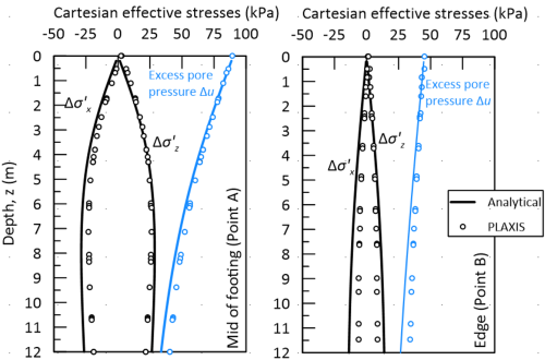
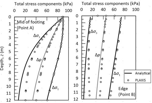
Let’s now see some typical results for the problem at hand (the relevant calculations are omitted for brevity). Figure 4.35 presents profiles of effective Cartesian stress increments and excess pore pressures with depth at the middle of the footing (Point A) and at its edge (Point B) immediately after application of the pressure, as well as profiles of total stress component increments with depth at the same locations. Results of the analytical expressions provided above are compared with the corresponding results of a PLAXIS model, developed to obtain the distribution of stresses in soil underneath the strip pressure shown in Figure 4.34 for the case of B = 16 m and H = 50 m. Good agreement is observed between stress computed with the two methods, particularly close to the surface (z = 0). There is a caveat though. The expressions provided above are for a soil profile of infinite depth, which cannot be simulated with a PLAXIS model. To obtain the results presented in the following, a 50m-thick soil layer was modelled in PLAXIS, and the bottom of the layer was fixed along both the horizontal and vertical direction. This fixity condition will affect the distribution of stresses, and consequently the predicted deformation profiles.
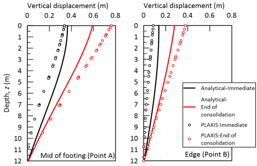
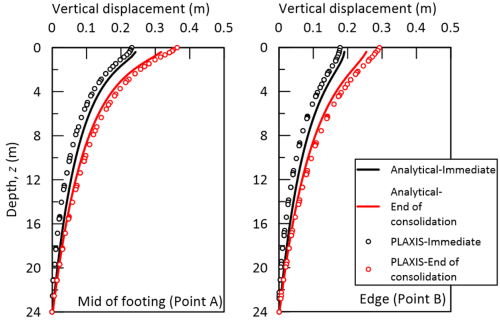
Profiles of vertical soil displacements at Points A and B immediately after application of the pressure and at the end of consolidation are presented in Figure 4.36. Analytical results are compared against results of a linear elastic PLAXIS simulation, considering this time B = 16 m and H = 12 m. Notice that, while the results of the analytical calculations and of the PLAXIS simulation are generally in agreement, they certainly do not match. The reason for that is the differences in the distribution of stresses that stem from the boundary conditions at the bottom of the soil layer: In PLAXIS we consider that an incompressible sandy layer is found at depth 12 m (Figure 4.34). While in the analytical calculations, even though we have considered only 12 m of soil, we are assuming that this soil layer is underlain by compressible material of infinite thickness. It is important to appreciate this limitation of hand calculations, that is not associated with modelling soil as linear elastic material. This suggests that the comparison between analytical results and PLAXIS will improve, as the dimensionless thickness of the layer H/B increases. Indeed, the gap between the predictions closes in Figure 4.37, which presents results for the same problem, but for H/B = 12 (case of B = 2 m wide footing on H = 24 m thick layer).
