4.5 Immediate settlement of shallow foundations

George Kouretzis

4.5 Immediate settlement of shallow foundations

Elastic settlement of soil subjected to uniform, flexible loadings can be simply calculated as the sum of the volumetric strains ε_vol along the thickness of the compressible layer, Η:

(4.7) $\rho = \int\limits_0^{\rm H} {{\varepsilon _{vol}}dz}$

The same basic concept applies for the estimation of settlement of shallow foundations. Nevertheless, we need to introduce some corrections in the above equation to account for the effect of the rigidity of the foundation, the embedment depth, and the shape of the footing, while appropriately considering drained or undrained conditions. These are discussed in the following paragraphs.

4.5.1 Effect of footing rigidity: Immediate settlement and contact stresses

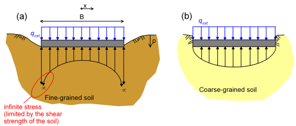
Distortion of soil due to the application of an external load or pressure depends on the rigidity of the loaded area, and the type of soil (fine-grained or coarse-grained) i.e., whether immediately after application of a loading the soil will behave as drained or undrained. In case of rigid footings (Figure 4.10), settlement is of course uniform. The distribution of contact stresses below the footing is, nevertheless, highly non-uniform. Assuming that soil behaves as elastic material, contact stresses at the outer edge of the footing (x = B/2, Figure 4.10) would become infinite:

(4.8) $\Delta {\sigma _z} = \dfrac{{2{q_{ext}}}}{\pi }\dfrac{1}{{\sqrt {1 - {{\left( {\dfrac{{2x}}{B}} \right)}^2}} }}$

In a real fine-grained soil however, they are limited by its shear strength. The drained Young’s modulus E′ of coarse-grained soils depends on the degree of confinement, and this affects the distribution of stress underneath a loaded area. The fact that the drained Young’s modulus E′ depends on the confining stress is mathematically expressed as:

(4.9) $E' = {E'_{ref}}{\left( {\dfrac{{p'}}{{{p_{ref}}}}} \right)^m}$

where p′ is the mean effective stress p′ = (σ′₁+σ′₂+σ′₃)/3, Ε′_ref is the reference modulus value at a reference mean stress p_ref, while the exponent m is considered usually m = 0.5 for sands and m = 1.0 for clays. In other words, the Young’s modulus is non-linear function of mean stress in sands. Near the outer edges, where confinement (i.e., the mean stress) is less compared to the centre of the footing, the stresses are lower (Figure 4.10b).

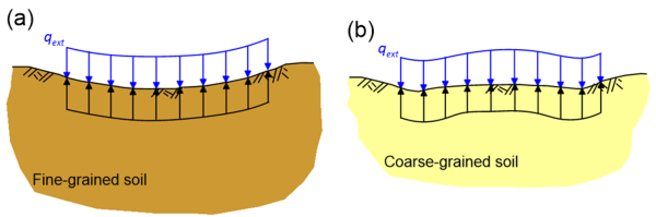
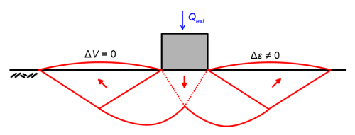
The image on the left depicts a rigid footing on fine grained soil. The footing is subjected to uniform pressure qext. The reaction stresses are infinite at the edges of the footing, and decrease towards to middle, where the minimum reaction stress develops. The image on the right depicts a rigid footing on coarse grained soil. The footing is subjected to uniform pressure qext. The reaction stresses are zero at the edges of the footing, and increase towards to middle, where the maximum reaction stress develops. — Figure 4.10. Distribution of contact stresses below a rigid footing transferring uniform vertical pressure to (a) fine-grained and (b) coarse-grained soil.

Contact stress distribution under a flexible loaded area is uniform, but the settlement profile varies as soil surface is free to deform, depending again on whether soil is fine-grained or coarse-grained (Figure 4.11). The shape of the deformed surface in the case of saturated clay (undrained loading) will be concave upward (Figure 4.11a), as it is reasonable to assume a uniform value of E_u across the thickness of the compressible clay layer, as in Figure 4.10a. On the other hand, the shape of the deformed surface in the case of a coarse-grained material (drained loading) will be concave downward (Figure 4.11b). That is because the Young’s modulus of sands E′ varies non-linearly with confining stress. As the latter are lower near the edge of the footing, compared to the stresses at its centre, the settlement developing near the edges will be higher than near the centre of the footing.

The image on the left depicts a flexible footing on fine grained soil. The footing is subjected to uniform pressure qext. The reaction stresses are uniform, and concave upwards. The image on the right depicts a flexible footing on coarse grained soil. The footing is subjected to uniform pressure qext. The reaction stresses are non-uniform, larger stresses develop towards the edges and lower stresses develop towards the middle. where the minimum reaction stress develops. The image on the right depicts a rigid footing on coarse grained soil. The footing is subjected to uniform pressure qext. The reaction stresses are zero at the edges of the footing, and increase towards to middle, where the maximum reaction stress develops. — Figure 4.11. Distribution of contact stresses below a flexible footing transferring uniform vertical pressure to (a) fine-grained and (b) coarse-grained soil.

4.5.2 Effect of embedment depth

The pressure acting on the soil that will result in ground settlement is the additional pressure Δq_extimposed at the level of the foundation, on top of the pre-existing geostatic vertical effective stress at this level, σ′_z₀. Settlement due to the stress σ′_z₀ has already taken place during soil deposition, before application of the loading.

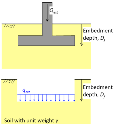
Schematic showing a footing embedded is soil with unit weight γ at depth Df and subjected to an external force Qext. For analysis purposes the footing is modelled as pressure qext applied at depth Df. — Figure 4.12. Effect of embedment depth.

If the foundation level is at the ground surface, and no other loads exist (e.g., preloading) then σ′_z₀ = 0 and the additional pressure Δq_ext is equal to the pressure from the footing q_ext i.e., the applied force divided by the area of the footing Q_ext/(Area). But in the common case where the topsoil is excavated for the construction of the foundation level at depth D_f (Figure 4.12) and soil is unloaded, the pre-existing vertical effective stress σ′_z₀ is equal to the geostatic stress at this level σ′_z₀ = γD_f_, where γ is the unit weight of the soil. In that case:

(4.10) $\Delta {q_{ext}} = {q_{ext}} - \gamma {D_f}$

Besides, embedment of a foundation will further reduce the expected settlement as:

Soil stiffness generally increases with depth. Foundation on a stiffer soil layer will of course result in less settlement.
Normal stresses from the soil above the foundation level increase confinement.
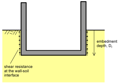
Part of the loading may be transferred through the side walls, as shear resistance can be mobilised at the soil-walls interface. Accommodation of part of the loading by side resistance reduces settlement (Figure 4.13).

Diagram illustrating the shear resistance developing at the wall of a foundation embedded in soil at depth Df. — Figure 4.13. Development of shear resistance at the soil-wall interface.

4.5.3 Drained or undrained soil response for calculating immediate settlements

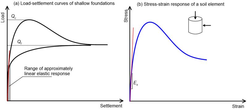
Methods for estimating settlement which are based on the theory of elasticity are often applied to predict settlement of structures founded on coarse-grained (sand, gravel) soils. We use such methods while considering the drained elastic parameters of soil i.e., the drained Young’s modulus E′ (also referred to as compressibility modulus, or deformation modulus) and the drained Poisson’s ratio v′. As soil behaviour is actually non-linear, the appropriate value of the Young’s modulus to be used with a method assuming linear elastic soil behaviour should take into account the stress levels that are expected to be applied in soil (Figure 4.14). Of course it is prudent to design the foundation so that strains in the foundation soil under serviceability conditions remain low, therefore elasticity formulas should provide a relatively good approximation of soil behaviour in situ. Furthermore, one should keep in mind that the Young’s modulus generally increases with depth, as it is a function of the mean stress level (see Section 4.5.1).

For fine grained soils, if the applied stress is sufficiently less than the yield stress of soil, immediate (short term) settlement should indeed be approximately linear elastic. In fact, the author could argue that good design practice requires designing any foundation or earthwork (embankment) so that the yield stress of soil (i.e., its preconsolidation stress, see Section 4.6.2) is not exceeded immediately after loading the foundation soil. In that case, we can apply methods for estimating settlements that are based on the theory of elasticity, while considering the undrained elastic parameters of the soil i.e., the undrained Young’s modulus E_u, which can be estimated from triaxial undrained tests in soil samples (Figure 4.15) and the undrained Poisson’s ratio v_u≈ 0.5, that satisfies the requirement for zero volume change during undrained loading. Remember that according to the theory of elasticity, the undrained Young’s modulus, for deformation under constant volume, is related to the drained Young’s modulus as:

(4.11) ${E_u} = \dfrac{3}{{2\left( {1 + v'} \right)}}E'$

The theory behind the above Eq. 4.11 is discussed in Chapter 4.7.

The figure on the left presents two load-settlement curves of shallow foundations: One curve exhibits hardening, and the ultimate load is denoted as Qf. The other curve exhibits softening, and the ultimate load is denoted as Qc. The range of approximately linear elastic response, at low strains, is indicated. The figure on the right presents the softening stress-strain curve of a soil sample subjected to triaxial loading. The soil Young's modulus Es is defined as the inclination of the curve at low strains. — Figure 4.14. (a) Load-settlement curves of shallow foundations, and (b) Stress-strain soil response.

Graph presenting the deviator stress-axial strain curve measured during a undrained triaxial compression test on a soil sample. The ultimate stress is denoted as 2Su. E_u^50 is defined as the secant modulus at deviator stress Su. It is noted that E_u^50=3G^50 — Figure 4.15. Estimation of the undrained Young’s modulus *E_u* (at a stress level equal to half the failure stress) from triaxial compression tests.

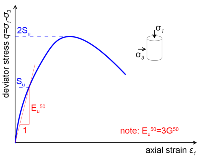
Keep also in mind that undrained loading under constant volume does not necessarily mean zero deformation, as it is the case of one-dimensional consolidation in the oedometer test. In two-dimensional problems, as the problem of predicting the immediate settlement of shallow footings, lateral soil heave is allowed to develop, and immediate settlement can occur under constant volume (see also Figure 4.9). This is also depicted in Figure 4.15, where undrained triaxial loading of a soil sample results in axial, but also lateral strains.

4.5.4 Immediate settlement of arbitrarily-shaped rigid footings on homogeneous half-space

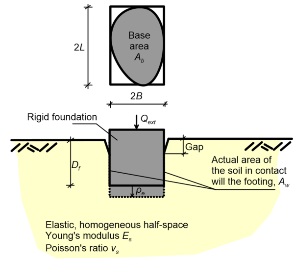
The immediate (elastic) settlement of rigid shallow footings of arbitrary shape can be estimated using the following expression by Gazetas et al. (1985), which is based on the assumption of linear elastic soil resting on a homogeneous half-space (Figure 4.16):

(4.12) ${\rho _e} = \dfrac{{{Q_{ext}}}}{{{E_s}L}}\left( {1 - \nu _s^2} \right){\mu _s}{\mu _{emb}}{\mu _{wall}}$

where: Q_ext is the vertical load (units: force) acting on the footing under serviceability conditions; E_s = E_uif the foundation soil is fine-grained (undrained conditions), or E_s = E′ if the foundation soil is coarse-grained (drained conditions). In that case Eq. 4.12 provides the total settlement; v_s = v_u ≈ 0.5 if the foundation soil is fine-grained (undrained conditions), or v_s = v′ if the foundation soil is coarse-grained (drained conditions); L is the half-length of the circumscribed rectangle.

Diagram illustrating a rigid foundation on an elastic half-space. The foundation is embedded at depth Df and is subjected to an external force Q_ext. The properties of the homogeneous half-space are Young's modulus Es and Poisson's ratio vs. A plan view of the foundation is used to define its width as 2B and its length as 2L. The base area is defined as A_b and the area of the soil in contact with the footing is defined as Aw. — Figure 4.16. Geometry to calculate settlement of rigid shallow footings (after Gazetas et al. 1986).

Moreover, μ_s is a factor accounting for the shape of footing, equal to:

(4.13) ${\mu _s} = 0.45{\left( {\dfrac{{{A_b}}}{{4{L^2}}}} \right)^{ - 0.38}}$

μ_emb is a factor accounting for the effect of embedment:

(4.14) ${\mu _{emb}} = 1 - 0.04\dfrac{{{D_f}}}{B}\left[ {1 + \dfrac{4}{3}\left( {\dfrac{{{A_b}}}{{4{L^2}}}} \right)} \right]$

μ_wall is a factor accounting for the effect of wall friction:

(4.15) ${\mu _{wall}} = 1 - 0.16{\left( {\dfrac{{{A_w}}}{{{A_b}}}} \right)^{0.54}}$

The parameters that appear in the above expressions are defined in Figure 4.16, while values of the ratio A_b/4L² for common footing shapes are presented in Table 4.3.

**Table 4.3.** Values of *A_b/*4L² for common footing shapes.
Footing shape	A_b/4L²
Square	1
Rectangle	B/L
Circular	0.785
Strip	0

This method is valid for “deep” homogeneous soil. In practice this means that the thickness of the surficial compressive layer should be larger than the influence depth of the load. If that is not the case, the method will result in (over)conservative settlement predictions, as discussed in Example 4.8. In addition, it is the author’s view that the factor accounting for the wall friction must be used with caution, as it is not at all certain that the interface’s shear strength will be mobilised at the wall-soil interface under the serviceability load. It is therefore reasonable to assume that μ_wall = 1 i.e., no load is transferred through friction.

Note that the method described above does not apply to strip footings, as it predicts infinite settlement. This is a consequence of assuming that the thickness of the compressible layer is infinite.

4.5.5 Immediate settlement of footings on fine-grained soil layer of limited thickness

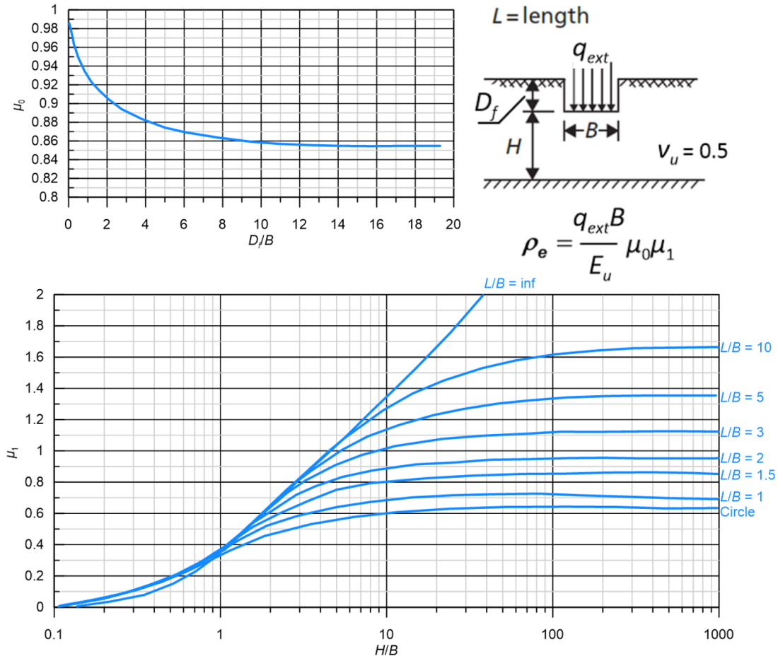
When the thickness of the compressible soil layer relatively to the dimensions of the foundation is relatively small, and the compressible soil is underlain by a practically incompressible layer, the method described in Section 4.5.4 will provide over-conservative settlement predictions. If the foundation soil is fine-grained, the immediate settlement of a flexible footing transferring pressure q_ext to a soil layer of finite thickness can be calculated according to Christian and Carrier (1978) as:

(4.16) ${\rho _e} = \dfrac{{{q_{ext}}B}}{{{E_u}}}{\mu _0}{\mu _1}$

where μ₀ accounts for the effect of embedment and μ₁accounts for the thickness of the compressible layer relatively to the dimensions of the footing (Figure 4.17). In addition B is the width of the footing and E_u is the undrained Young’s modulus of the fine-grained soil. Note that Figure 4.17 depicts values of μ₀ and μ₁ that correspond to Poisson’s ratio v_u= 0.5, hence the above are valid only for undrained loading conditions.

The figure on the top presents the variation of the factor μ_0 with the embedment ratio Df/B. The figure on the bottom presents the variation of the factor μ_1 with the thickness ratio H/B, for different values of L/B ranging from circle to inf. An inset figure is used to define the width of the footing as B, the embedment depth as Df, and the thickness of the compressible layer measured from the embedment depth as H. The soil Poisson's ratio is v_u=0.5. — Figure 4.17. Coefficients μ₀ and μ₁ for Poisson’s ratio v_u=0.5 (after Christian and Carrier 1978).

License

Icon for the Creative Commons Attribution 4.0 International License

Fundamentals of foundation engineering and their applications Copyright © 2025 by University of Newcastle & G. Kouretzis is licensed under a Creative Commons Attribution 4.0 International License, except where otherwise noted.