2.7 Mechanisms of contaminants transport through soil
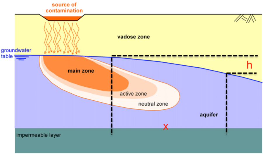
When a pollutant escapes from a repository, it moves through the vadose zone, which is the zone between the soil surface and the groundwater table (Figure 2.10). The soil grains retain part of the pollutant, either chemically or mechanically, while part of the pollutant reaches the aquifer. Water-soluble pollutants are then carried away downstream, following the groundwater flow, which is determined by the hydraulic gradient.
As pollutants are being carried away, contamination of the aquifer spreads and substance concentration decreases, as we move from the main zone to the neutral zone (Figure 2.10). Especially for saturated or partially saturated soils and pollutants that can be dissolved or suspended in water (light NAPLs that float are excluded), three basic mechanisms can be identified:
2.7.1 Advection or Hydraulic transportation
The contaminant is carried away by the groundwater though the soil voids, following the hydraulic gradient (Figure 2.10). Assuming saturated flow, the seepage velocity will be equal to:
(2.1) 
where n is the soil porosity (n=Vvoids/V) and q is Darcy’s water flux, equal to the volume Q flowing though a unit cross-sectional area A:
(2.2) 
In Eq. 2.1 k is the permeability of the aquifer, h is the hydraulic head, i is the hydraulic gradient and x defines the flow direction (Figure 2.10). Based on the above the adjective mass flux of the contaminant, defined as the mass flowing through a unit cross-sectional area per time (units: mass/(time length2)), is given as:
(2.3) 
where c is the concentration of the contaminant in the liquid phase. The concentration c in a specific location constantly varies with time, while concentration in a specific volume of water remains constant, as this volume of water flows following the hydraulic gradient.
2.7.2 Diffusion or molecular diffusion
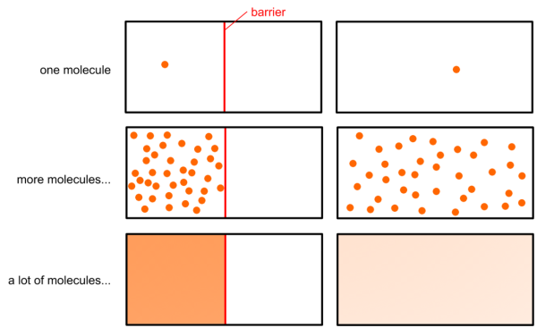
Contrary to advection transport, which refers to macroscopic movement, diffusion is a molecular based phenomenon. The contaminant is diffused in the groundwater, due to variation in concentration, meaning that the substance moves from areas of high to areas of low concentration. Figure 2.11 illustrates this from a microscopic and macroscopic point of view. Initially there are solute molecules (or ions) of the contaminant only on the left side of a barrier. These molecules or ions move randomly. As a result of this motion, if we remove the barrier, the solute diffuses to fill the whole container, moving from the high concentration area (left) to the low concentration area (right). Diffusion will continue until the concentration of the contaminant becomes equal everywhere. The rate at which these irregularities in concentration disappear can be quantified via Fick’s first law of diffusion:
(2.4) 
Eq. 2.4 suggests that the diffusive mass flux of the contaminant Jdiffusion, which provides the mass of the contaminant flowing through a unit cross-sectional area per time (units: mass/(time length2)), depends on the difference in concentration, the inverse of the distance, and a diffusion coefficient D. This is a function of the type of cation, temperature, soil porosity and soil tortuosity. In other words, diffusion of the contaminant does not depend on groundwater flow, and can take place in still water too.
2.7.3 Dispersion or mechanical dispersion
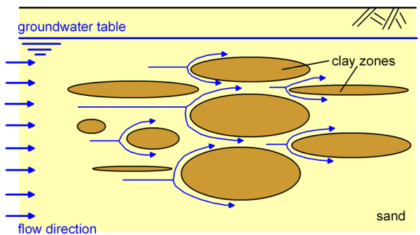
Movement of the contaminant is due to the presence of interconnected voids of the soil skeleton, of various shapes. Thus in microscopic scale, the velocity of water moving though the voids varies from place to place (Figure 2.12), and may diverge from the mean (macroscopic) groundwater flow i.e., the substance can be transported perpendicularly to the macroscopic groundwater flow too. Similar to the diffusion mechanism described above, the dispersive mass flux of the contaminant Jdispersion provides the mass of the contaminant flowing through a unit cross-sectional area per time:
(2.5) 
Jdispersion (units: mass/(time length2)) depends again on the difference in concentration, the inverse of the distance, and a dispersion coefficient Dd, which is a function of the seepage velocity and of the longitudinal dispersivity.
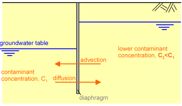
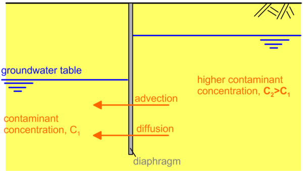
Often, these mechanisms may act antagonistically (Figure 2.13) or simultaneously (Figure 2.14). More specifically, the advection mechanism tends to transport the contaminant from right to left, from the area of high hydraulic potential to the area of lower hydraulic potential, following the hydraulic gradient. The diffusion mechanism on the other hand tends to transport the contaminant from the area of high concentration to the area of low concentration (Figures 2.13 and 2.14).
Therefore to calculate the evolution of contaminant concentration with time we need to solve the continuity Eq. 2.6, which describes mathematically the transport of a conserved quantity (here the mass of the contaminant):
(2.6) 
where m is the mass density (mass of contaminant per unit volume), J is the mass flux vector considering the above mechanisms and S quantifies the increase (S > 0) or reduction (S < 0) of the contaminant mass. Positive S terms are referred to as “sources” and negative S terms are referred to as “sinks”.
The gradient of the mass flux vector:
(2.7) ![\nabla J = \dfrac{{\partial J}}{{\partial x}}i + \dfrac{{\partial J}}{{\partial y}}j + \dfrac{{\partial J}}{{\partial z}}k,{\rm{with \: \:}}\hat i = \left[ {\begin{array}{*{20}{c}}1\\0\\0\end{array}} \right]{\rm{ }}\hat j = \left[ {\begin{array}{*{20}{c}}0\\1\\0\end{array}} \right]{\rm{ }}\hat k = \left[ {\begin{array}{*{20}{c}}0\\0\\1\end{array}} \right]](https://oercollective.caul.edu.au/app/uploads/quicklatex/quicklatex.com-33b3e5e36d4d3ea64a75b573bc3f6bdf_l3.png "Rendered by QuickLaTeX.com")
will provide the direction towards which the mass flux vector rises faster in the three-dimensional space, and its magnitude provides a measure of how fast the mass flux rises in this direction. For example, if the mass flux vector due to advection and diffusion is J = -3x-4y where x is the horizontal axis and y is the vertical axis, then:
(2.8) 
Other, non-mechanical mechanisms may also act to reduce and disperse the pollution load, and are introduced as “sinks” in Eq. 2.6:
- Chemical interaction, referring to the absorption of pollutants on the surface of clay particles or, ion exchange between pollutants and clay particles.
- Biological and biochemical reactions, such as the disintegration of organic pollutants by microorganisms.
- Nuclear procedures, such as particle decay.
