1.7 The Cone Penetration Test (CPT)
A very common method for in situ testing of soils is the Cone Penetration Test (CPT). A cone is hydraulically pushed into the soil at a constant rate, and the resistance to the penetration of the cone, as well as the frictional resistance of a surface sleeve, are continuously recorded. Today the piezocone test (CPTu) is more common, where pore pressure is also measured during penetration. Other variants allow for the measurement of S- and P- wave velocities (seismo-cone), moisture content, soil pH etc. A detailed description of the Cone Penetration Test procedure presented herein is included in AS1289.6.5.1.
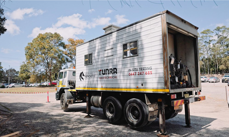
The Cone Penetration Test provides a continuous profile of soil stratigraphy, and allows also for continuous evaluation of soil properties; contrary to the SPT test where information about the soil penetration resistance is obtained at specific intervals. However, soil samples for visual inspection and laboratory index testing are not retrieved, as with the SPT test. CPT tests can be performed in very soft clays to dense sands alike, onshore and offshore (Figure 1.21). In addition, Cone Penetration Testing is often used in other geotechnical engineering applications, such as estimating the liquefaction potential of loose coarse-grained deposits.
However, CPT is unsuitable for gravelly soils, cemented soils and soft rocks, as the cone cannot penetrate through such formations. Some of the advantages and disadvantages of the CPT test are summarised in Table 1.6.
During a CPT sounding, the following quantities are measured:
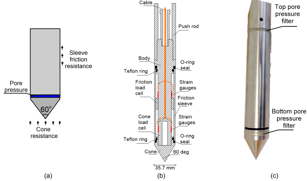
- The cone resistance qc (units: stress), which results from dividing the total force acting on the cone Fcone by the projected area of the cone, Ac (Figure 1.22).
- The sleeve friction resistance fs (units: stress) which results from dividing the total friction force acting on the sleeve Fsleeve by the area of the sleeve, Αs (Figure 1.22).
The diameter of standardised cones is 35.7 mm, and their projected area is Ac = 1000 mm2.
| Advantages | Disadvantages |
|---|---|
| Continuous profiling | No soil samples are retrieved, estimates of soil type are indirect |
| Economical and productive. 100 m to 350 m/day, depending on equipment and soil conditions | High capital investment |
| Results are not operator-dependent | Requires skilled operator |
| Many interpretation methods based on rigorous theoretical background, and not just empiricism | Requires calibration, noise filtering as well as careful instrument preparation e.g., saturation of pore pressure sensor (tensiometer) |
| Particularly suitable for soft soils as well as applications such as assessment of seismic liquefaction potential | Unsuitable for fills, gravel/boulder deposits and cemented soils |
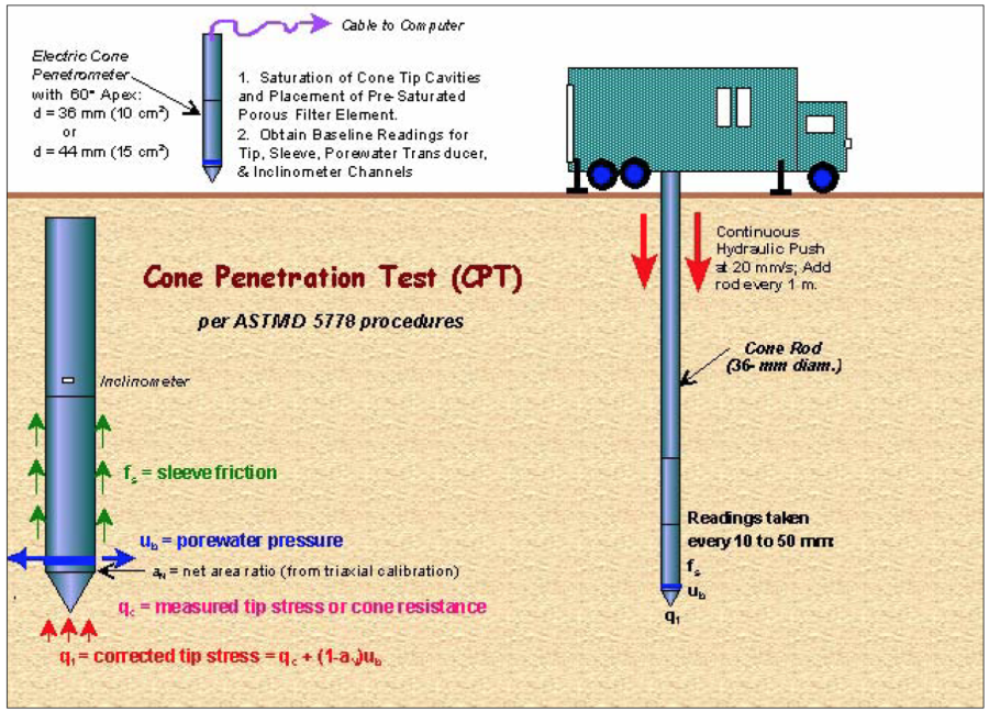
CPT testing (Figure 1.23) must follow some standarised procedures (AS1289.6.5.1):
- To avoid damaging the cone when penetrating through artificial compacted fills or surficial hard soils, pre-drilling might be necessary.
- The cone thrust direction should be as near as possible to vertical. Its deviation, measured by means of an inclinometer installed on the rig, should not exceed 2 deg.
- Reference measurements must be obtained, and zero forces on the cone should be recorded at the start and at the end of each CPT sounding.
- The rate of penetration of the cone should range between 10 to 20 mm/sec. This implies that a 20 m CPT sounding can be completed in about 30 min, and excess pore pressures will develop during CPT tests in low permeability soils (Figure 1.24).
- Measurements must be obtained at 25 mm to 35 mm intervals for soil under a pavement or for design of pavement depth, or every 150 mm to 200 mm for any other application. This is the minimum interval prescribed in the standard, more frequent measurements are obtained with modern equipment.
- During a pause in penetration, any excess pore pressure generated around the cone will start to dissipate. The rate of dissipation depends on the coefficient of consolidation, and thus the permeability of the soil. Dissipation tests can be performed in fine grained soils at any depth to get estimates of permeability, by measuring the decay of excess pore pressures with time.
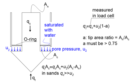
- When CPTu tests are performed in saturated soft clays and silts, the cone resistance qc must be corrected to account for the pore water pressure acting on the cone geometry as: qt = qc+u2(1-a) where u2 is the measured pore water pressure and a is determined from calibration tests (Figure 1.25). Generally, the tip area ratio a ranges between a = 0.70 to 0.85, and should not be less than a = 0.75.
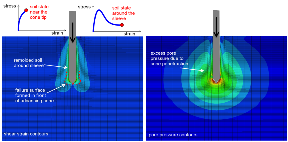
Interpretation of CPT tests is based on theoretical considerations regarding the properties of the failure surface that continuously develops near the cone tip (and around the sleeve) as the cone is being advanced into soil. While interpreting CPT tests one must consider that i) the soil near the cone tip reaches its peak shear strength, while ii) the soil’s residual strength associated with large shear strains is mobilised around the sleeve.
Considering the above, the variation with depth of the following quantities is calculated (Figure 1.26), according to AS1289.6.5.1:
The cone resistance qc (kPa), determined as:
(1.6) 
where Fcone is the force acting on the cone tip (kN), measured by means of a load cell (cone strain gauge load cell, Figure 1.22b), and mg is mass of the inner rods at the test depth (kg).
If necessary (i.e., in CPTu tests), cone resistance is corrected for pore pressure development, according to the mentioned above:
(1.7) 
Note that we may use the symbols qc and qt interchangeably: qc refers to cone resistance from CPT tests, and qt refers to cone resistance from CPTu tests, which has been correct for pore pressure effects.
The sleeve friction resistance fs (kPa), determined as:
(1.8) 
where Fsleeve is the force on the sleeve, equal to the total force on the cone and sleeve (measured by means of the friction strain gauge load cell, Figure 1.22b) minus the force on the cone alone (kN), and As is the surface area of the friction sleeve (mm2).
The friction ratio (%), which is equal to:
(1.9) 
and the pore water pressure u2, measured via a pore pressure transducer installed above the tip of the cone in CPTu rigs.
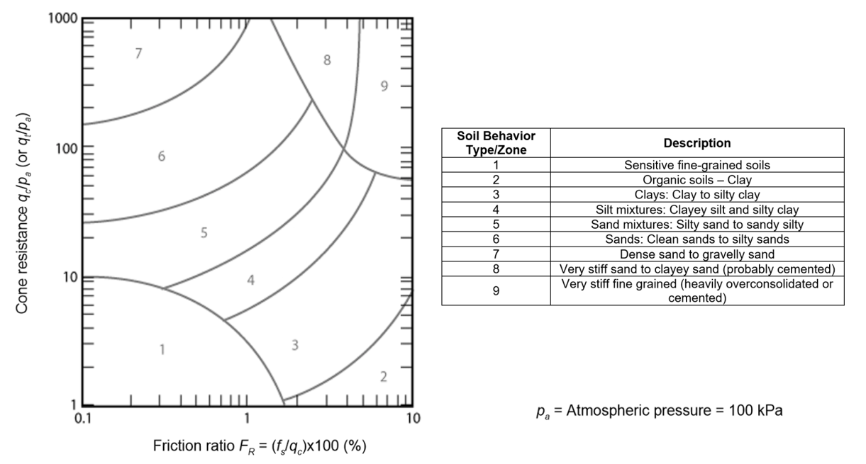
One of the main applications of the CPT test is the indirect determination of subsoil stratigraphy i.e., the thickness of soil layers and the soil type. As a rule-of-thumb, the cone resistance qc is high in sands and low in clays, and the friction ratio FR is high in clays (3% < FR < 10%) and low (0.5% < FR < 1.5%) in sands. It was mentioned before that we cannot obtain soil samples from the CPT test for laboratory characterisation tests. Thus, the CPT test cannot provide direct characterisation of the soil based e.g. on its grain size distribution, but rather of the Soil Behavior Type (SBT), a quantity which can be correlated to its mechanical characteristics (Robertson and Kabal, 2022). The Soil Behavior Type is determined from the chart presented in Figure 1.27, based on the dimensionless cone resistance measured at a particular depth, divided against the atmospheric pressure qc/pa (or qt/pa, if applicable), and the corresponding friction ratio FR at the same depth from Eq. 1.9.
A disadvantage of the soil stratigraphy interpretation method described above is that it does not account for the increase in cone resistance and sleeve friction resistance with overburden stress, as the cone is being pushed deeper into the soil. To alleviate this, interpretation methods based on normalised cone resistance and sleeve friction resistance have been proposed. Such a procedure is described in Robertson and Kabal (2022). First, the normalised cone resistance Qtn is calculated as:
(1.10) 
where σ′z0 is the effective vertical geostatic stress at the depth where each cone resistance measurement qt is obtained, pa is the atmospheric pressure and Cc is a correction factor similar to that of Eq. 1.2, calculated as:
(1.11) 
where n ≤ 1.0 is an exponent provided by the following expression:
(1.12) 
The factor Ic is the so-called Soil Behaviour Type index, and is calculated as:
(1.13) 
where Fr (%) is the normalised sleeve friction resistance:
(1.14) 
where σz0 is the total vertical geostatic stress at the depth where each cone resistance and sleeve friction measurement is obtained. As it is clear from the above expressions, Qtn must be calculated iteratively, by assuming an initial value of the exponent n e.g., n = 1 and iterating until the change in n between successive iterations becomes less than Δn = 0.01.
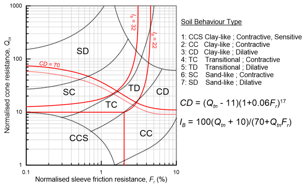
Accordingly, Figure 1.28 (Robertson and Kabal 2022) can be used to obtain the Soil Behaviour Type, as well as an estimate of the behaviour of non-cemented soils at large strains (dilative or contractive). CD in Figure 1.28 defines the boundary between contractive and dilative behaviour, while IB is a modified Soil Behaviour Type index that defines the transition zone between sand-like and clay-like behaviour via an intermediate (transitional) soil zone.
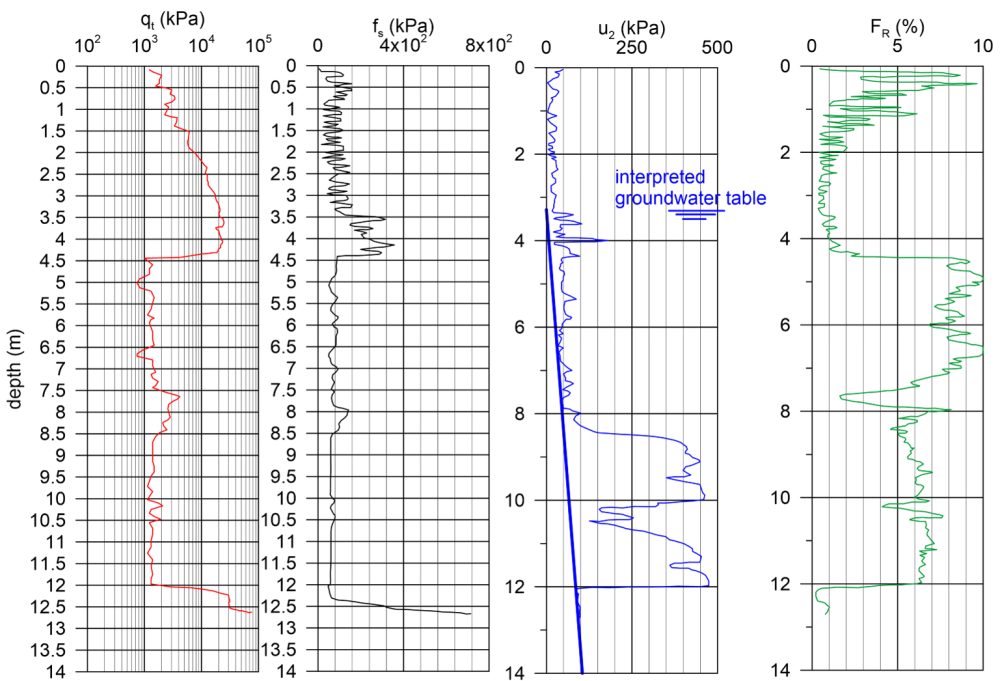
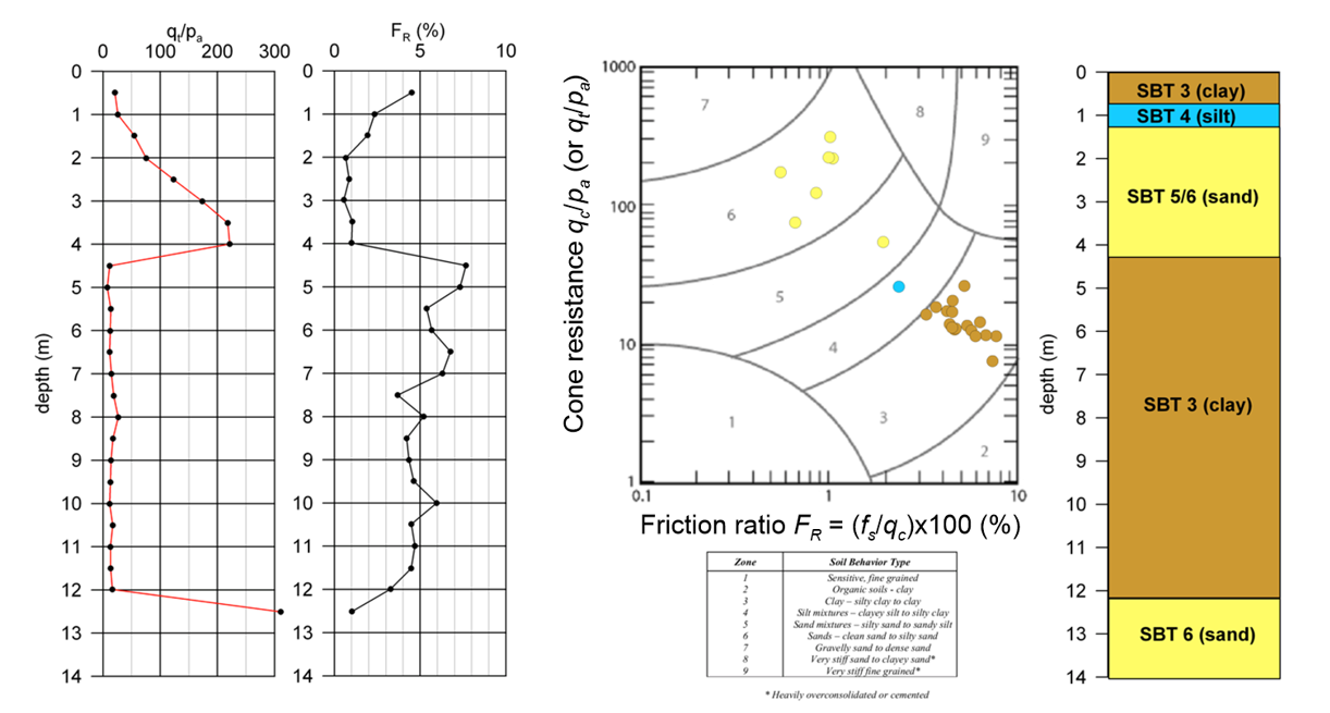
An example soil behavior type profile determined with the method depicted in Figure 1.27 is presented in Figure 1.29. Different dots in the soil behavior type chart correspond to different cone resistance/friction ratio pairs, depicted from their distribution with depth on the left. Depending on the zone of the chart where each dot lies, a SBT is assigned to each pair, and a different color is used. Using the distribution of SBT with depth, different layers can be identified along the soil profile, as presented on the right. Although it is clear that CPT provides a more “objective” evaluation of the soil profile, based on the SBT chart, engineering judgment is always necessary to interpret a rational soil stratigraphy.
