3.7 Discussion
While applying the expressions presented in the above paragraphs, one should keep in mind that stress increments due to external loadings are total stresses, and initially will be resisted by both the pore water pressure and the soil skeleton. As discussed in Part 4, settlement in soils is due to effective stress changes only.
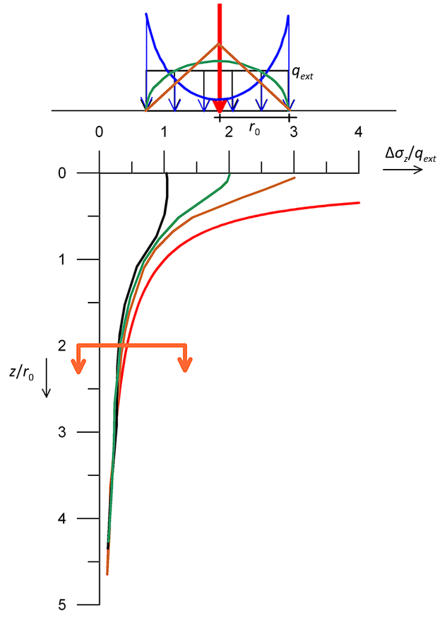
Application of these solutions can be extended to treat more complex loadings, under specific conditions: The Saint-Venant principle (1855) suggests that “the difference between the effects of two dissimilar but statically equivalent loadings becomes very small at sufficiently large distances from the loading”. Consider for example the different stress distributions presented in Figure 3.11, and assume we are interested in estimating soil stresses at a depth equal to about the diameter of the loaded area 2r0 (Figure 3.11). From that depth and below, stresses in soil depend on the magnitude of the resultant of the loading, and not on its distribution. In other words, in certain cases we can use elasticity theory expressions even if the actual distribution of the loading is not the same as the idealised uniform distribution, provided that the resultant is the same.

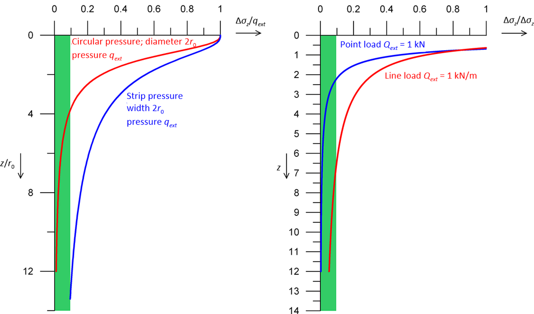
The expressions provided in the previous paragraphs for the calculation of vertical stress increments with depth due to various loading types can be applied for the determination of the influence depth of the loading, defined as the depth where additional vertical stress Δσz is reduced to 10% of the mean stress applied on the soil surface (Δσz/qext = 0.1).
Plotting the distribution of the additional normalised (against the pressure applied on the surface qext) stress with depth below the axis of symmetry of a circular area, and of a strip pressure with equivalent width (Figure 3.12a), we determine the influence depth to be:
(3.16)  for uniform pressure on a circular area of radius r0
(3.17)  for strip pressure of width B = 2r0
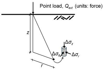
Similarly, plotting in Figure 3.12b the distribution of the additional normalised vertical stress with depth below the axis (r = 0, Figure 3.5) of a point load, provided from the expression:
(3.18) 
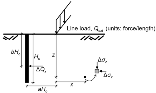
and below the axis (x = 0, Figure 3.6) of a line load, provided from the expression:
(3.19) 
we determine the influence depth to be 2 m for the point load, and 6.5 m for the line load.
The above findings may prove to be very useful for the preparation of a finite element model, for determining the extent of the geometry that must be simulated to accurately consider the effects of an external loading.

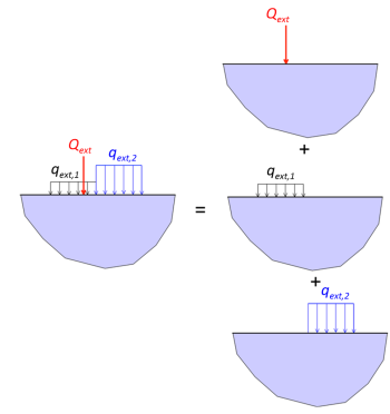
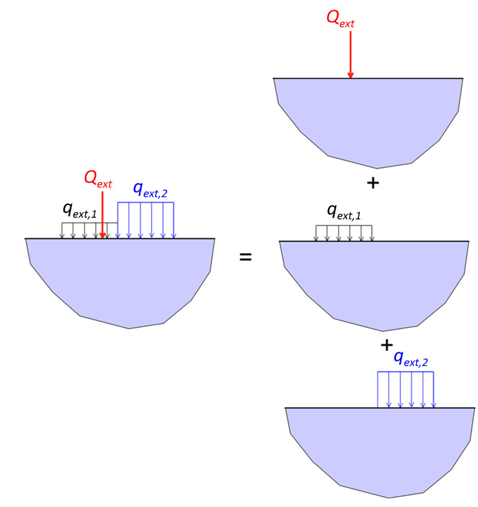
Another advantage arising from the consideration of the soil as a linear elastic material is that the principle of superposition applies. This suggests that stress increments due to multiple loadings acting simultaneously can be calculated as the sum of stress increments due to each one of the loads or pressures considered separately as (Figure 3.13):
(3.20) 
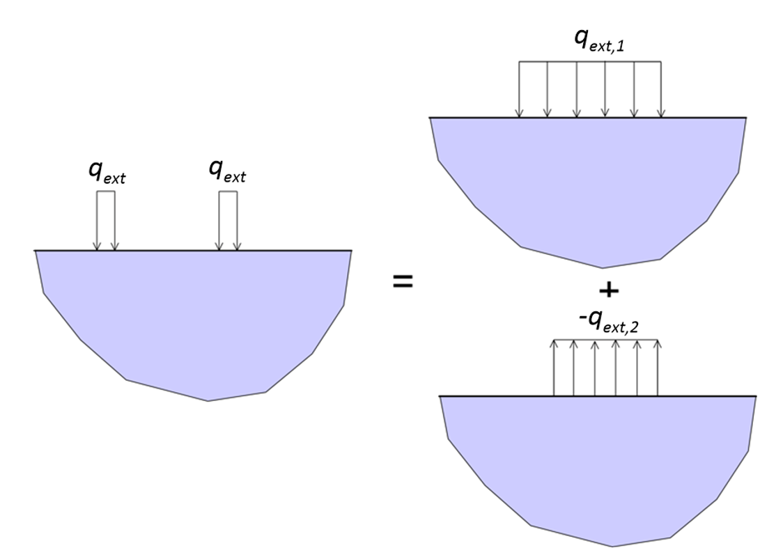
Stresses resulting from other, more complex loading distributions can be also calculated, if “negative”, tensile loadings are considered together with compressive loadings (Figure 3.14). This concept is demonstrated in Example 3.1.
(3.21) 

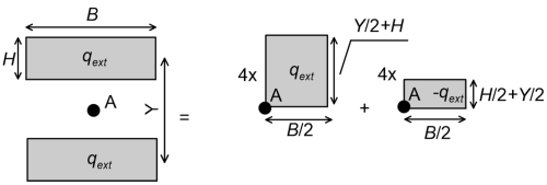
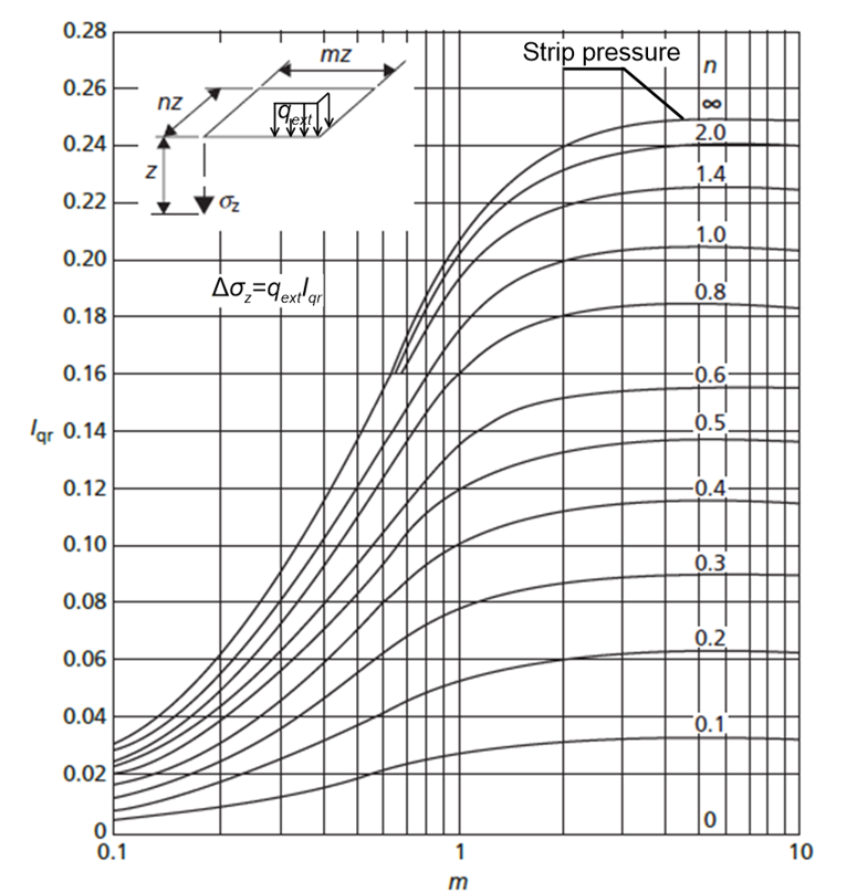
Figure 3.10 also can be used in tandem with the principle of superposition to obtain vertical stress increments underneath complex pressure distributions. For example, Figure 3.15a demonstrates how we can calculate vertical stress increments underneath point A, located midway from two rectangular areas of dimensions H × B separated by distance Y on which pressure qext is applied e.g., underneath the tracks of a piling rig. The vertical stress increment at any depth at point A due to the two rectangular pressures shown in Figure 3.15a is equal to four (4) times the vertical stress increment at the edge of a rectangular pressure qext of dimensions (Y/2+H) × B/2 minus four (4) times the vertical stress increment at the edge of a rectangular pressure qext of dimensions (Y/2+H/2) × B/2. Vertical stress increments at the edge of rectangular pressures are calculated directly from Figure 3.10.
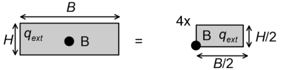
Similarly, Figure 3.15b demonstrates how we can calculate vertical stress increments underneath point B, located at the centre of a rectangular area of dimensions H × B on which pressure qext is applied e.g., underneath the centre of a rectangular footing. The vertical stress increment at any depth at the centre B of a rectangular pressure qext of dimensions H × B is equal to four (4) times the vertical stress increment at the edge of a rectangular pressure qext of dimensions Y/2 × B/2, calculated according to Figure 3.10.
To end with, it should be noted that all the solutions presented above were derived for “flexible” loads and pressures, and do not account for the rigidity of the foundation. If the foundation is rigid, stress increments for the same loading on the surface would be generally lower by 15% to 30%. However, usually we do not correct stress distribution for the rigidity of the footing since, as soil non-linearity is not taken into account, we prefer the “error” to be on the conservative side.
