3.1 Introduction to Part 3
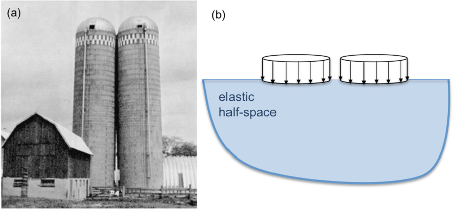
Consider the following practical problem: Two storage tanks are going to be founded on a layer of stiff saturated clay. Due to restrictions related to the cost of land, the Geotechnical Engineer is called to find the minimum distance that the silos can be placed apart. Keep in mind that when two foundations are placed too close to each other, stresses imposed to the soil will overlap, with (sometimes) detrimental consequences (Figure 3.1a). In order to provide an answer to the above practical question, we must find a way to calculate the magnitude of stresses that a foundation imposes in soil, and its area of influence i.e., the area where these additional stresses are significant.
Stress distribution in soil due to external loadings can be determined analytically, while considering a simplified geometry of the foundation (Figure 3.1b), and the soil to be a homogeneous, isotropic and linear elastic material.
But unquestionably soil is not an elastic material. So why do we use linear elasticity theory to calculate stresses? There are three main reasons for that:
- There are practical cases where soil actually behaves “elastically”. For example, settlement of a foundation is estimated while considering the working load (serviceability conditions), which should be a fraction of the collapse load. For settlement to remain within the tolerable limits, soil should remain effectively in the elastic region (Figure 3.2).
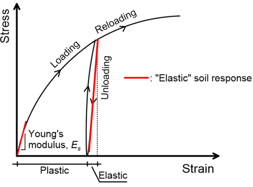
Figure 3.2. Elastic response of soils during loading and unloading.
- Calculation of stresses (but not strains) is not particularly sensitive to material properties. For example, consider the uniaxially loaded sample made of any material (not necessarily soil) depicted in Figure 3.3. The axial stress σz will depend on the magnitude of the load Q and the area of the sample A, and is independent of the material properties. However, the axial and lateral strains εz and εx respectively, will depend on the material properties, namely the Young’s modulus Es and the Poisson’s ratio, vs.
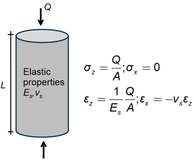
Figure 3.3. Calculation of stresses and strains in an uniaxially loaded material sample.
- Simplicity. Considering soil to be a linear elastic material implies that only two (independent) soil parameters, determined via soil testing, will be involved in the calculations: the soil’s Young’s modulus Es and its Poisson ratio νs. On top of that, Poisson’s ratio is not particularly sensitive to the type of soil, and ranges between vs = 0.2 to 0.5.
Based on the above, we can use analytical, closed-form solutions and charts to determine the distribution of stresses in soil, which are much easier and straightforward to apply compared to e.g., numerical analyses. Formulas for simple, characteristic load and pressure distributions are presented in the following chapters, considering idealised two-dimensional axisymmetric and plane-strain symmetry conditions.
It is reminded here that plane-strain symmetry corresponds to loading and geometry conditions where the out-of-plane dimension of the structure under consideration is large compared to the dimensions of its cross-section (Figure 3.4a), thus we can assume that the out-of-plane displacement and strain are both equal to zero.
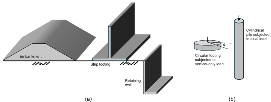
A two-dimensional plane-strain model may be used to simulate a continuous strip footing, a pipeline, a retaining wall or an embankment.
Axisymmetric conditions on the other hand correspond to cases of rotational symmetry about the vertical axis of the problem, where the radial displacement in cylindrical coordinates is zero uθ = 0 (Figure 3.4b). A two-dimensional axisymmetric model may be used to simulate a circular footing subjected to uniform vertical force, a pile subjected to a compressive or tensile vertical force, or a triaxially loaded soil sample. Keep in mind that both geometry and loading symmetry must co-exist e.g., the case of a laterally loaded pile or a horizontal force applied on a circular footing are rather three-dimensional problems, as contrary to the geometry, the loading is not symmetric.
In the following Chapters, we will use the term load to describe external forces (Qext) acting on soil, and the term pressure to describe external pressures (qext) acting on soil. Loading(s) is a general term, referring to both forces and pressures.
