2.10 Design of a pollutant containment installation
As explained in Section 2.8.1, impermeable barriers can be used in conjunction with a dewatering system to lower the phreatic line underneath a pollutant source, and thus prevent contamination of the groundwater. Design of such a system requires, among others, to verify whether the capacity of the dewatering system to be installed is sufficient for lowering the water table to the desired level. Given the complexity of this problem, it is not possible to use analytical methods. This example demonstrates the use of the Finite Element method for the design of a pollutant containment installation.
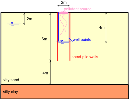
A schematic of the considered problem is shown in Figure 2.29. The width of the pollutant source is 2 m, and its length is assumed to be sufficiently larger than its width, so that the problem can be treated as two-dimensional plane strain (Part 3). Two parallel rows of sheet piles spaced at 2 m apart are driven into soil up to a depth of 6 m, and will act as impermeable barriers containing the pollutant source. The subsoil profile is the same as Chapter 2.9, and consists of a 10 m-thick homogeneous and isotropic silty sand layer of permeability 1 m/day, underlaid by an impermeable silty clay layer.
The in situ groundwater table is found at 2 m depth, and a dewatering system will be installed, to lower the groundwater table by 2 m underneath the pollutant source. The proposed dewatering system consists of a series of dewatering well points (spears) along the length of the pollutant source. The capacity of the pumping system is 0.4 m3/day/m.
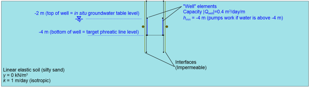
An outline of the numerical model used to simulate this problem is shown in Figure 2.30. As in Chapter 2.9, the silty sand is modelled as weightless linear elastic material. The compressibility parameters of the material are irrelevant, as only a steady state flow analysis is performed. The silty clay layer is not modelled explicitly, instead flow is not permitted from the bottom of the model, to simulate the existence of that impermeable layer. The sheet pile walls are not explicitly modelled either, instead interfaces with zero cross permeability along their 6 m length are introduced to simulate containment of the pollutant zone by means of driving of sheet piles walls.
The dewatering spears are simulated by vertical one-dimensional “well” elements, extending from the elevation of the in situ groundwater table (-2 m) to the target phreatic line beneath the pollutant source (-4 m). The well elements require two input parameters. The first is their capacity, in m3/day per unit length of the pollutant source along which the line of spears is to be installed. In this example we set the capacity to be 0.4 m3/day/m, and we will explore whether this capacity is sufficient to lower the groundwater table to the target phreatic line elevation. The second parameter is the elevation hmin, which is the minimum depth where the pumps extract water from. This is set to be equal to the target phreatic line elevation, which means that water will be pumped from the spears if the water level is at 4 m or above. The lateral boundaries of the model are placed at sufficient distance from the area of interest, so that the existence of the free flow boundary conditions there will not affect the results of the simulation (see Chapter 2.9).
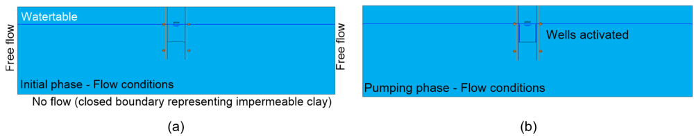
As in Chapter 2.9, the analysis consists of two steady-state groundwater flow-only phases: During the initial phase we define the in situ groundwater table level and the flow conditions at the boundary (Figure 2.31a), and the software calculates the initial pore pressure profile. During the pumping phase we activate the wells and the interfaces (Figure 2.31b) while leaving the flow boundary conditions and the global water table level unchanged. Again, the phreatic line shown in Figure 2.31b is not the final but rather the target one. The final one will result from the calculation. Note that the model cluster between the interfaces is not deactivated here, as no soil is excavated.
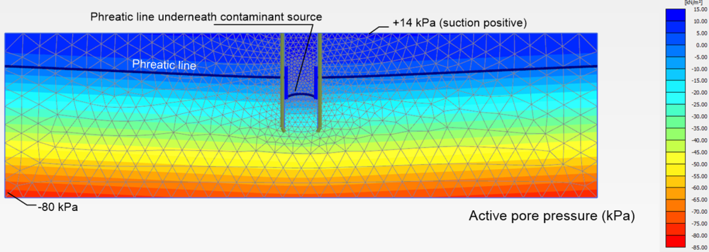
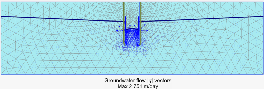
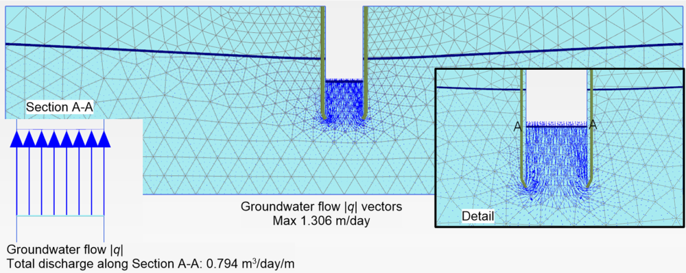
Key outcomes of this analysis are presented in Figure 2.33. Pore pressure contours are plotted together with the phreatic line resulting from steady-state pumping through the spears in Figure 2.32a. Inspection of the phreatic line underneath the contaminant source suggests that the capacity of the pumps is sufficient to achieve the desired lowering of the groundwater table. The predicted phreatic line level is of course sensitive to the distance between the sheet piles walls (or the wells). As in Chapter 2.9, positive pore pressures indicating suction are calculated above the phreatic line.
Finally, groundwater flow vectors are presented together with the finite element mesh in Figure 2.32b. Unlike Chapter 2.9, the maximum groundwater flow vectors are not observed at the toe of the sheet pile walls (Figure 2.28), but rather at the bottom of the wells, where potential seepage failure will develop in this case. The magnitude of the groundwater flow depends again on the length of the impermeable sheet piles, and will be reduced if the sheet piles are embedded in larger depth.
