2.9 Design of a pump-and-treat installation

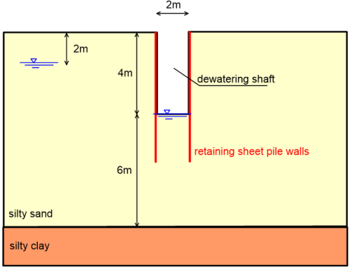
This chapter presents the use of the Finite Element method (computer code PLAXIS) to determine the capacity of water pumps required to dewater a 2 m wide by 30 m long shaft (Figure 2.24) used for the extraction of contaminated groundwater. The presented method is applicable to the design of any dewatering system when two-dimensional plane strain conditions apply i.e., when the width of the dewatered area is much longer than its length (see Part 3).

This problem involves modelling of steady state flow, and can be solved analytically using flow net-based methods under certain conditions i.e., uniform homogeneous and isotropic soil, with equal permeability k along both the horizontal and vertical directions. However, while for most soils the permeability along the vertical direction is not much lower than the permeability along the horizontal direction, the assumption of uniform soil conditions is rarely met in situ. Such assumptions are not required when using numerical methods to solve steady state flow problems.

Consider the soil conditions illustrated in Figure 2.24 where the shaft is excavated in a 10 m-thick silty sand layer of permeability k = 1 m/day (vertical permeability equal to horizontal permeability). The sand layer is underlain by a silty clay layer that can be considered as impermeable. Whilst the stability of the retaining system is not studied in this example, the length of the (assumed impermeable) sheet pile walls will affect flow of groundwater into the shaft (thus the hydraulic gradient i) and must be considered in the analysis. For the problem at hand, we assume that the minimum length of the sheet pile walls required to retain the excavation is equal to 6 m. Finally, the groundwater table is found at 2 m from the ground surface, and the target pump capacity should be such that the bottom of the excavation remains dry.

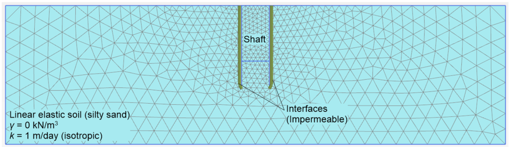
An outline of the numerical model and of the finite element mesh is presented in Figure 2.25. Only the 10m-thick silty sand layer is modelled, and the existence of the impermeable silty clay layer is considered by setting the bottom horizontal boundary of the model to be impermeable. The lateral boundaries of the model are placed at sufficient distance from the area of interest (shaft) so that boundary conditions will not affect the calculated flow into the shaft. Good practice suggests performing a sensitivity analysis with respect to the distance of the lateral boundaries from the area of interest, to confirm that results are not compromised by boundary effects. Sand is modelled as linear elastic material, however the unit weight of the material and its elastic properties (Young’s modulus, Poisson’s ratio) will not affect the results of the particular analysis, as displacements are not considered-only a steady state groundwater flow analysis is performed. Finally, the sheet pile walls are not explicitly modelled, as the structural properties of the retaining system are not of interest here. Instead, we model the retaining system by modelling two “interfaces” along the edges of the shaft, of length equal to the length of the sheet pile walls (6 m). These interfaces are assigned zero cross permeability (impermeable), although it is possible to model some flow through the retaining system.

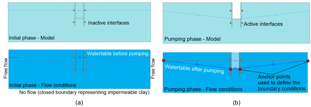
The analysis phases are presented in Figure 2.26. During both stages we model only flow (Calculation type: “Flow only”) and calculation of pore pressures is based on “Steady state groundwater flow”. The initial stage (Figure 2.26a) is used to calculate pore pressures before excavation and dewatering of the shaft. As such, the global water table is set to be horizontal, at 2 m from the ground surface. Free flow is allowed from the lateral boundaries, while no flow is allowed from the bottom boundary representing the impermeable clay layer. The interfaces are not active at this stage. It must be noted here that positive pore pressure values will be calculated above the water table with this model, representing suction in the unsaturated soil zone. While this does not affect the calculations described here, it is important to obtain a realistic suction profile if stability of the excavation is to be modelled too, as suction will affect soil strength and compressibility. This can be achieved by selecting a proper water retention model for soil, such as the Van Genuchten model, and allocating appropriate parameters to it.

The second analysis stage (Figure 2.26b) models lowering of the water table due to pumping inside the shaft, and will provide the total flow inside the shaft when the groundwater table is lowered at its bottom by means of pumping. As such, the geometry cluster representing soil inside the shaft must be de-activated, to model excavation of soil. At the same time the interfaces are activated, to account for zero horizontal flow from the sheet pile walls. The target phreatic line is input, as shown in Figure 2.26, by setting the water table level to be at 2 m from the surface at the lateral boundaries, and at 4 m from the surface inside the shaft. Note that this is not the actual phreatic line, the geometry of the phreatic line during steady state pumping will result from the analysis. Flow conditions at the boundaries remain unchanged, and are inherited from the initial stage.

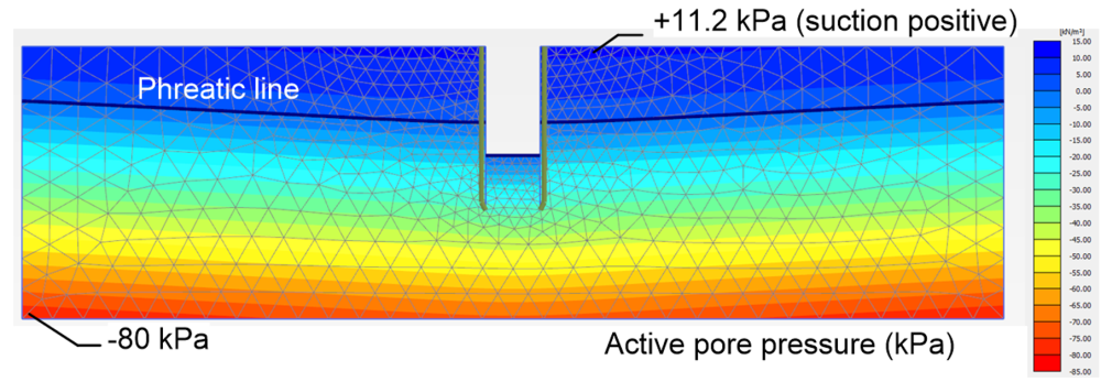
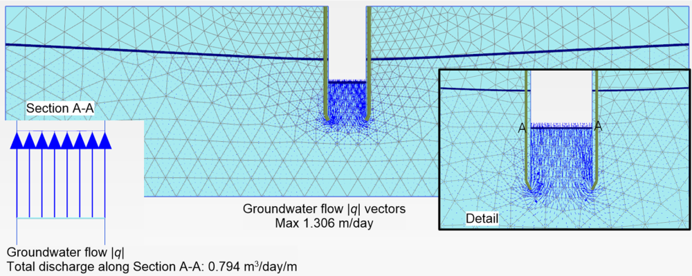
Some key results from the analysis are shown in Figures 2.27 and 2.28. Figure 2.27a presents the phreatic line during steady state pumping and the active pore pressure contours. Notice that while the pore pressure at the elevation of the silty clay layer is equal to the hydrostatic pressure near the lateral boundaries (80 kPa), notable suction values are calculated above the phreatic line, as explained earlier. The required pumping capacity can be determined by plotting groundwater flow vectors (Figure 2.28) and finding the total discharge into the shaft along the cross section A-A, at the bottom of the shaft. Since the total discharge through the bottom of the shaft is 0.794 m³/day/m, the required capacity of pumps to be installed in the 30 m-long shaft is 30×0.794 = 23.8 m³/day.

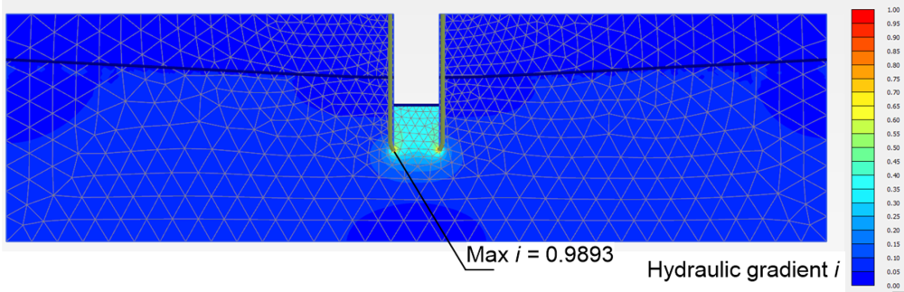
However, notice in Figure 2.27b, which presents hydraulic gradient contours, that the maximum hydraulic gradient in soil underneath the excavation is near unity. It is reminded that the critical hydraulic gradient i_cr, required for sand “boiling” i.e., seepage failure to occur is:

(2.12)

where γ′ is the submerged unit weight of soil, γ_w is the unit weight of water, G_s is the specific gravity of soil (G_s = 2.65 for most silica-based soils) and e is the void ratio. The critical hydraulic gradient is of the order of i_cr = 1 for most soils, which suggests that failure of the excavation due to seepage is very possible in this case, if the specific retaining system is adopted.

This issue can be alleviated by increasing the length of the sheet pile walls, thus the energy consumed during flow of water underneath the sheet pile walls. Indicatively, an increase in the length of the sheet pile walls by 3 m (9 m long sheet pile walls in total) results in decrease of the maximum hydraulic gradient from i = 0.989 to i = 0.637. Increasing the length of the retaining system will of course result in reducing the required capacity of the pumps, from 23.8 m³/day to 13.9 m³/day. These calculations demonstrate the importance of considering flow effects in the design of retaining systems in high permeability materials, when high groundwater table conditions are present.