Example 6.6

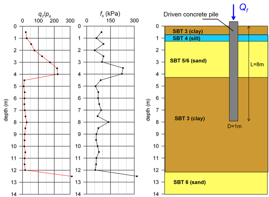
Estimate the ultimate geotechnical strength Q_f of the driven concrete pile shown below. The pile is subjected to axial compressive load and is embedded in a layered profile comprising both fine-grained and coarse-grained layers. Use CPT-based methods of Schmertmann (1978) and Bustamante and Gianeselli (1982) (Chapter 6.12) together with the CPT results provided below. Ignore the weight of the pile in the calculations.

Answer:

As discussed in Chapter 6.12, the correction factor α′ used in Schmertmann’s method in the determination of the skin friction resistance Q_sf of the pile depends on the nature of the surrounding soil (coarse-grained or fine grained). Thus, before proceeding with the estimation of the skin friction resistance, the soil behavior types SBT encountered along the length of the pile must be determined, according to the mentioned in Chapter 1.7.

1. Calculation of skin friction resistance Q_f using the method proposed by Schmertmann (1978):

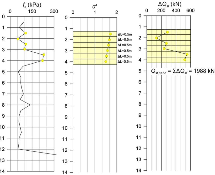
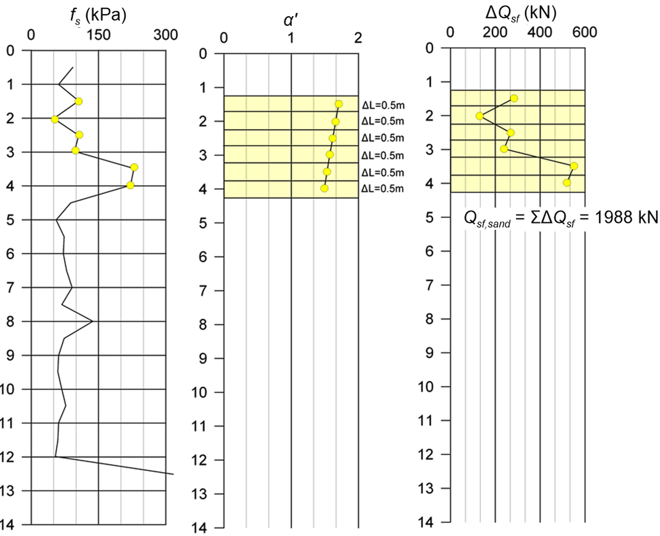
1.1 Skin friction resistance along pile shaft embedded in sand (SBT 5/6):

For the part of the concrete pile that is embedded into sand, the variation of the correction factor α′ with depth z is determined with the aid of Eq. 6.24 (Figure 6.55):

The sand layer is divided into sublayers, the thickness ΔL of which depends on the frequency of sleeve friction resistance f_s measurements from the CPT test.

The unit friction resistance of each sublayer ΔQ_f is then estimated with Eq. 6.23 (Figure 6.55):

and summed to find the skin friction resistance of the pile that develops along the part of the shaft embedded in the sand layer, Q_sf,sand.

Alternatively, we can use the Bustamante and Gianeselli’s method to estimate Q_sf,sand. In that case the skin friction resistance along each sublayer is calculated as f_sf = q_c/α where the coefficient α is provided by Table 6.6 for sand with q_c > 12 MPa (generally q_c/p_a > 120 in the provided data indicating dense sand) and driven precast concrete piles (Category IIA) to be α = 150. The limiting value of f_sf is from Table 6.6 f_sf < 120 kPa. Using the provided q_c values we calculate Q_sf,sand = 823 kN. There is significant difference between the results of the two methods, and is attributed only partly to the Bustamante and Gianeselli’s method imposing a limiting value to f_sf, as the f_sf is exceeded in merely two sublayers.

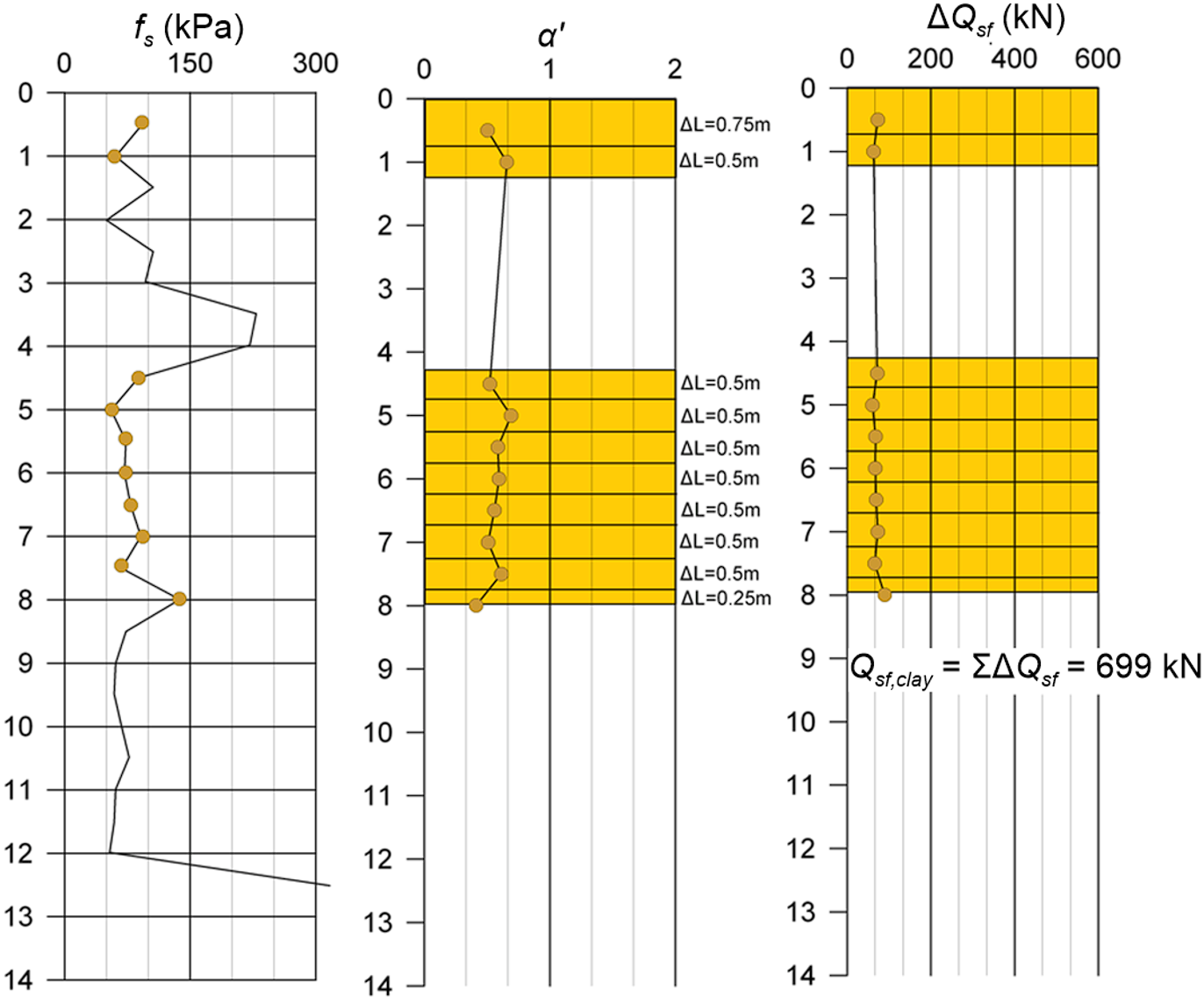
1.2 Skin friction resistance along pile shaft embedded in clay (SBT3) and silt (SBT4):

A similar procedure is followed for the part of the pile embedded into the fine-grained clay/silt layers. In that case, the correction factor α′ depends on the sleeve friction resistance, and is provided from Eq. 6.26 for concrete piles (Figure 6.56):

Dividing again into sublayers we can estimate the unit skin friction resistance with Eq. 6.23, and the total friction resistance developing along the part of the pile embedded in fine-grained soil, Q_sf,clay (Figure 6.56).

Again we will use the Bustamante and Gianeselli’s method to estimate Q_sf,clay, for comparison purposes. Skin friction resistance along each sublayer is again calculated as f_sf = q_c/α where the coefficient α for clay with q_c = 1 to 5 MPa (firm to stiff clay) and driven precast concrete piles (Category IIA) to be α = 40. The limiting value of f_sf is from Table 6.6 f_sf < 35 kPa. Using the provided q_c values we calculate Q_sf,clay = 499 kN. Again, there is a significant difference between the results of the two methods.

While this comparison is based on fictitious CPT data, therefore one may argue that the differences between the two methods may have been exaggerated (the total skin friction resistance estimated with Schmertmann’s method is Q_sf = 2700 kN, and the total skin friction resistance estimated with Bustamante and Gianeselli’s method is Q_sf = 1322 kN i.e., less than half) its purpose in not to endorse one method over the other. Instead, its purpose is to inform the reader about the uncertainties associated with estimating the ultimate geotechnical strength with empirical methods. This is the reason why careful selection of risk ratings AS2159 is required, particularly when using legacy methods to estimate the design bearing capacity of piles.

2. End-bearing resistance, Q_b:

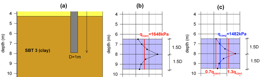
In order to apply the LCPC method and use Eq. 6.29 to estimation the end bearing resistance of the pile, we must first estimate the equivalent average cone resistance q_c(eq), following the procedure described in Chapter 6.12:

• Consider the cone tip resistance q_c within a range of 1.5D = 1.5 m below the pile toe to 1.5D = 1.5 m above the pile toe (Figure 6.57b) and calculate the average value of q_c(av) = 1648 kPa within this zone.
• Eliminate q_c values that are higher than 0.7q_c(av) and lower than 1.3q_c(av) (Figure 6.57c) and calculate q_c(eq) = 1482 kPa by averaging the remaining q_c values.

Furthermore, as the pile toe is embedded in clay, the empirical bearing capacity factor to be introduced in Eq. 6.29 is k_b = 0.6 according to Briaud and Miran (1991). Substituting in Eq. 6.29 yields:

We can perform a sanity check here, if we consider that the undrained strength of clays is correlated to the cone resistance with Eq. 1.16 as:

If we take an average N_kt value N_kt = 15 and an estimate of the total vertical stress at -8 m i.e. σ_z = 16 x 8 = 128 kPa we calculate at the base of the pile S_u,b = 90 kPa, which is reasonable for a stiff clay. Using Eq. 6.9 to calculate the end bearing resistance with the α-method we obtain:

Such “sanity checks” are particularly important, when empirical methods are employed for the design of piles.

3. Ultimate geotechnical strength, Q_f:

The collapse load of the pile is the sum of its skin friction resistance along the clay/silt and the sand layers, and end-bearing resistance:

 (using Schmertmann’s method to calculate Q_sf)

 (using Bustamante and Gianeselli’s method to calculate Q_sf)