Example 6.4

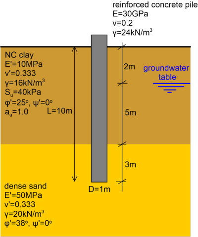
Determine the short-term and long-term load-displacement curve of the pile shown below, up to a maximum vertical pile head displacement of 30% of the diameter of the pile.

Answer:

The general concept described in Example 6.3 regarding the simulation of soil-pile interaction applies in this problem too. Note however that when considering drained loading conditions, for the clay layer under long-term loading and for the sand layer under both short-term and long-term loading, the interface strength reduction factor R_int will depend on the friction angle of the soil. For a concrete pile, where the interface friction angle φ_i is assumed to be equal to 2/3 of the soil friction angle φ′:

Geostatic effective stresses must be calculated, as an effective stress analysis (ESA) is performed when considering drained material behavior and groundwater is present. We can use the Undrained (B) Mohr-Coulomb material to simulate undrained clay response under short-term loading conditions, which allows for direct input of the undrained shear strength S_u while estimating effective stresses too. Notice that the drained Young’s modulus E′ and Poisson’s ratio v′ must be used in tandem with the Undrained (B) Mohr-Coulomb model. However, since here we are not interested in excess pore pressure development, using the Undrained (C) Mohr-Coulomb model for the clay will essentially yield the same results.

Under long-term loading conditions on the other hand, both clay and sand response are simulated with the Drained Mohr-Coulomb model, assuming non-associated flow (ψ = 0°) as per the brief. Although the effective cohesion of the normally consolidated clay and dense sand is equal to zero (c′ = 0), a small value of cohesion (c′ = 1 kPa) is considered with the Drained Mohr-Coulomb model, for numerical stability reasons. A linear-elastic material is used to simulate the pile, with Young’s modulus E_p = 30 GPa and Poisson’s ratio v_p = 0.2.

As in the Example 6.3, the analysis is performed in 3 stages:

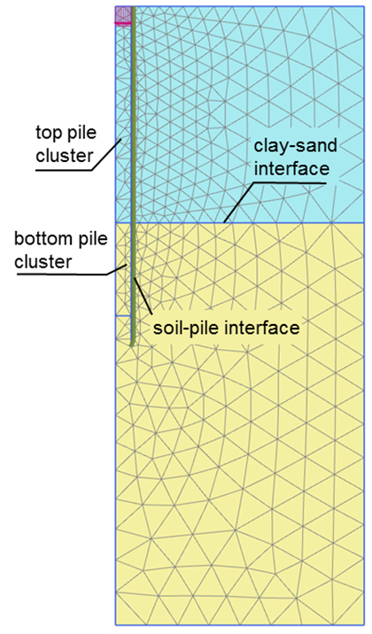
1. Initial stage (before the construction of the pile) Calculate initial geostatic stresses before the construction of the pile, by associating all geometry clusters with the original soil material. This means that two separate geometry clusters must be defined for the pile, connected at the interface of the soil-sand layers (Figure 6.52). Interfaces and loads are not active during this stage. Note that also PLAXIS uses Eq. 6.16 for the estimation of the lateral earth pressure coefficient Κ₀ and the lateral geostatic stresses.
2. Plastic stage 1 (construction of the pile) The material of the geometry cluster corresponding to the pile is switched to the linear elastic material described above, and interfaces are activated. This simplified procedure implies that the soil around the pile is not disturbed from its construction i.e., the pile is “wished in-place”.
3. Plastic stage 2 (loading of the pile) The prescribed vertical displacement u_y,f = 0.3D on the pile head is activated, and the analysis is run until it reaches the desired value.

Here, the groundwater table level must be explicitly introduced during the definition of the analyses stages. Geostatic effective stresses can be checked with hand calculations. Note that when we are using the Undrained (C) Mohr-Coulomb model for the clay, PLAXIS cannot compute effective stresses in this particular layer. However, as friction resistance in the clay layer does not depend on the effective stress level, the results will be essentially correct.

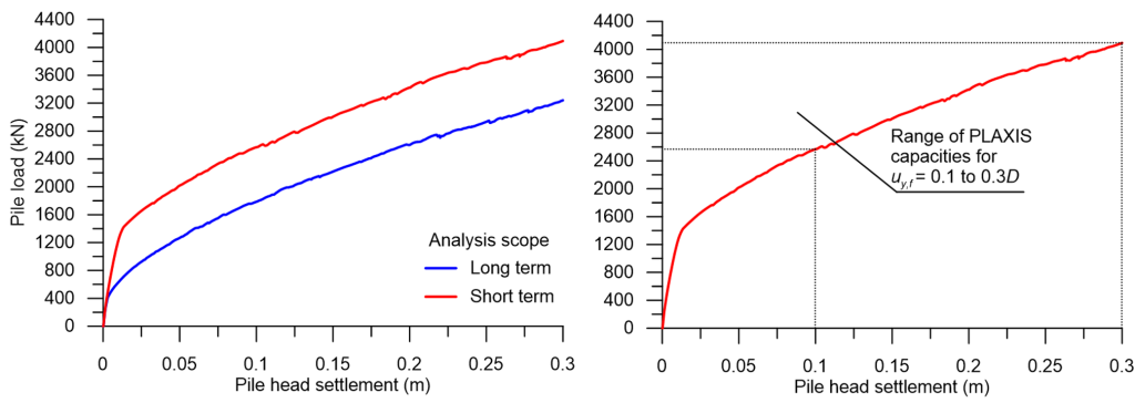
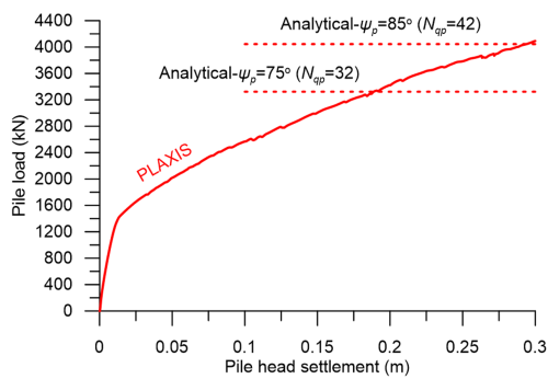
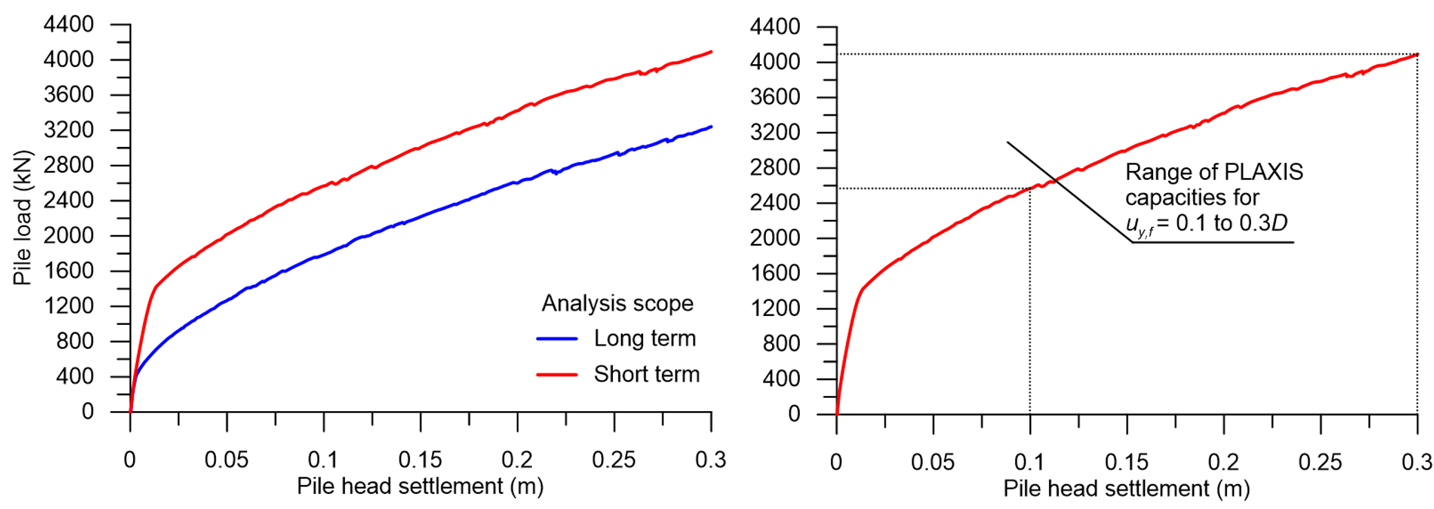
The load-displacement curves obtained from both the short-term and long-term analyses are presented in Figure 6.53, while the results of the short-term analysis are compared to the ultimate geotechnical strength estimated via the analytical α– and β-Method formulas in Figure 6.54. The upper bound of the collapse load was obtained while considering Eq. 6.20 and ψ_p = 85º for the bearing capacity factor N_qp, and the lower bound while considering ψ_p = 75º. The resulting bearing capacity factors are compatible with the recommendations in Table 6.4. Notice in Figure 6.53 that, as expected, the difference between the short-term and long-term response is solely due to the increased shaft friction under short-term conditions: when the maximum shaft friction resistance is reached, for a relative low pile displacement according to the mentioned in Chapter 6.7, the two load-displacement curves become parallel. As in the Example 6.2, long-term response is found to be critical for the design of the pile. As explained in Example 6.3, this is not a surprise: PLAXIS uses the same Coulomb model as the α– and β-methods to calculate interface shear stresses, and installation effects are customarily ignored i.e., the normal stress acting at the soil-pile interface is taken equal to the geostatic horizontal stress. Therefore, the simplifications introduced in the estimation of skin friction resistance in the α– and β-methods are carried over to PLAXIS, as it is based on the same interface strength model.

Finally, notice in Figure 6.53 that, unlike Example 6.3, here the selected nominal vertical pile head displacement associated with the collapse load has profound impact on the predicted value of the later. That is because the pile toe is now embedded in drained material (sand), which shear strength depends on the confining stress. As settlement of the pile upon loading results in the development of significantly high confining stresses under its toe, the limiting end-bearing pressure increases significantly as pile head settlement progresses and this is reflected to the load-displacement curve.

In such cases it is advised to carefully select the nominal vertical pile head displacement at failure, if a numerical model is used to estimate the collapse load: the nominal vertical pile head displacement at failure u_y,f should be the vertical pile head displacement that will result in failure of the structure supported by the pile, at the ultimate limit state.