Example 6.3

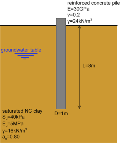
Determine the load-displacement curve (compliance curve) of the pile shown below, up to a maximum pile head vertical displacement equal to 30% of the diameter of the pile.

Answer:

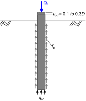
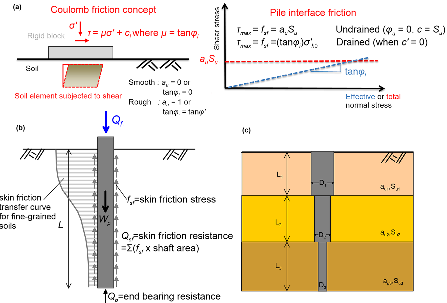
Installation of the pile is not going to be simulated, although this would be possible, but with a more complex numerical model. It is perhaps clear that, as the vertical load on the pile increases, shear stresses f_sf develop at the soil-shaft interface, and eventually some slippage will develop, as illustrated in Figure 6.45. Following the development of slippage at the soil-pile interface, stresses are being transferred to the pile toe, and reach the end bearing resistance q_bf at a vertical pile head displacement u_y,f that is taken between 0.1 and 0.3D (Figure 6.45). It has been mentioned earlier that modern CPT-based method associate the development of the end bearing resistance with a pile head displacement about u_y,f = 0.1D. Here we will explore, among others, how much the collapse load of the pile (the reaction at the corresponding displacement value, taken from the load-displacement curve) increases if we take the pile head displacement at failure u_y,f to be 0.3D, instead of 0.1D. It is reminded that analytical formulas (α– and β-method) assume that soil is rigid-plastic, hence pile head displacement at failure has no physical meaning.

When applying the α-method formulas, we used the conceptual model depicted in Figure 6.17 to determine the skin friction resistance at the pile-shaft interface, assuming that the full friction at the interface has mobilised:

In PLAXIS, and other numerical codes, interfaces are used to model soil-pile interaction. An interface describes the contact between two different model entities e.g. the soil and a pile, a retaining wall or a tunnel, and sometimes the interface of two different soil layers. The roughness of the interface, and thus the maximum shear stress that can develop along the interface before slippage occurs, is introduced in PLAXIS via the interface strength reduction factor (R_int). The contact interface model implemented in PLAXIS is based on the Coulomb friction criterion.

Considering again a rigid block resting on a surface, as in Figure 6.17, we can estimate the maximum shear stress at the interface when slip occurs as:

where φ_i and c_i is the friction angle and the cohesion of the interface, and are associated with the drained c′ and φ′ or undrained S_u shear strength properties of the soil layer, as:

and under drained conditions, or

under undrained conditions

for the pile problem at hand it is:

so

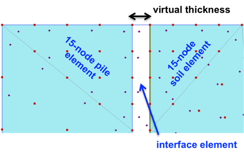
Each interface is assigned a virtual thickness, an imaginary dimension related to the average element size with the virtual thickness factor. The default PLAXIS value of 0.1 will provide reliable results for most problems. Interface elements are created by PLAXIS when an interface is defined, connecting the two adjacent regions (Figure 6.46).

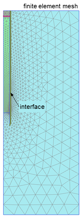
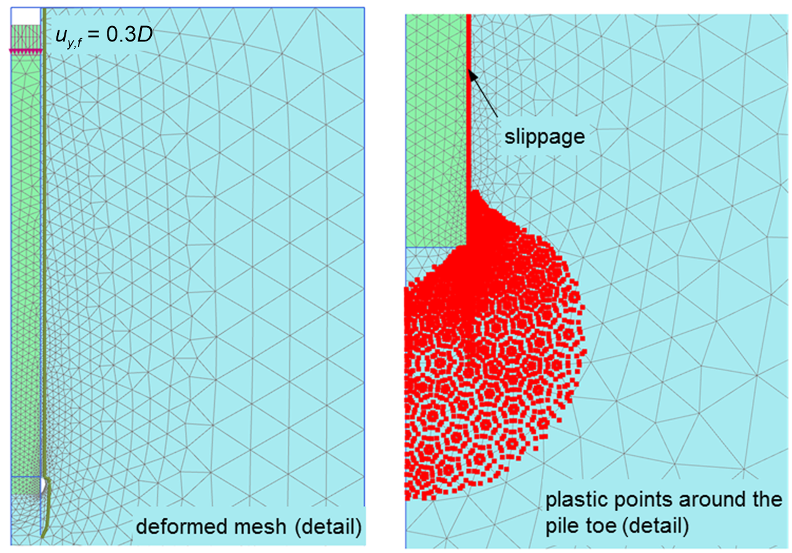
The axisymmetric finite element mesh is presented in Figure 6.47, with the axis of symmetry being the pile vertical axis. An area of dimensions 6 m x 16 m is discretised with a “medium coarse” mesh. A uniform prescribed displacement u_y,f is applied on the head of the pile, equal to 0.30D = 0.3 m, in order to obtain the compliance (load-displacement) curve of the pile.

The clay is simulated as an Undrained (C) Mohr-Coulomb material (Example 5.2), and a total stress analysis is performed. The interface reduction factor R_int = a_u = 0.8 is introduced to PLAXIS as a property of the soil material that interacts with the pile. A linear-elastic material is used to simulate the pile, with Young’s modulus E_p = 30 GPa and Poisson’s ratio v_p = 0.2. Note here that we can introduce the weight of the pile in the calculations, by assigning a proper unit weight to the pile’s material. Following Section 6.9, in PLAXIS simulations we do take into account unloading of soil during pile construction, because we assign the pile material to the soil column during Stage 2 of the analysis. Therefore, additional loading of soil associated with the self-weight of the pile results from the different in the unit weight of the soil column (γ = 16 kN/m³) and of the pile column (γ = 24 to 25 kN/m³ for reinforced concrete pile).

The analysis is performed in 3 stages:

1. Initial stage (before the construction of the pile) Calculate initial geostatic stresses before the construction of the pile with the “K₀ procedure”, by associating both geometry clusters with the clay material. Interfaces and loads are not active.
2. Plastic stage 1 (construction of the pile) The material of the geometry cluster corresponding to the pile is switched to the linear elastic material described above, and interfaces are activated. This simplified procedure implies that the soil around the pile is not disturbed from its construction i.e., the pile is “wished in-place”.
3. Plastic stage 2 (loading of the pile) The displacement on the pile head is activated, and the analysis is run until it reaches the desired value.

As in Example 6.1, while performing a total stress analysis (TSA) the groundwater table level will not affect the calculations, and does not need to be simulated.

A detail of the deformed mesh and of the plastic points near the area of the pile toe are plotted in Figure 6.48. Notice that slippage at the soil-pile interface develops, resulting in yielding of the soil elements around the shaft, while a failure zone develops below the pile toe.

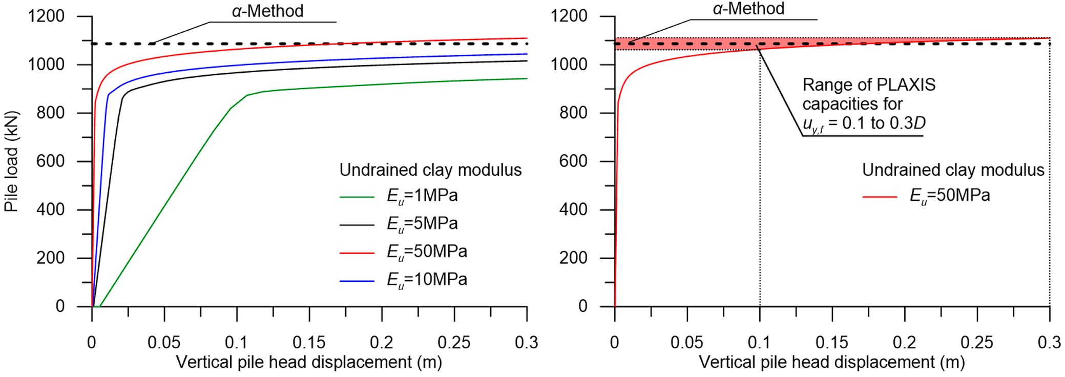
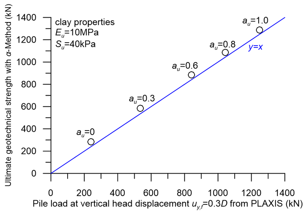
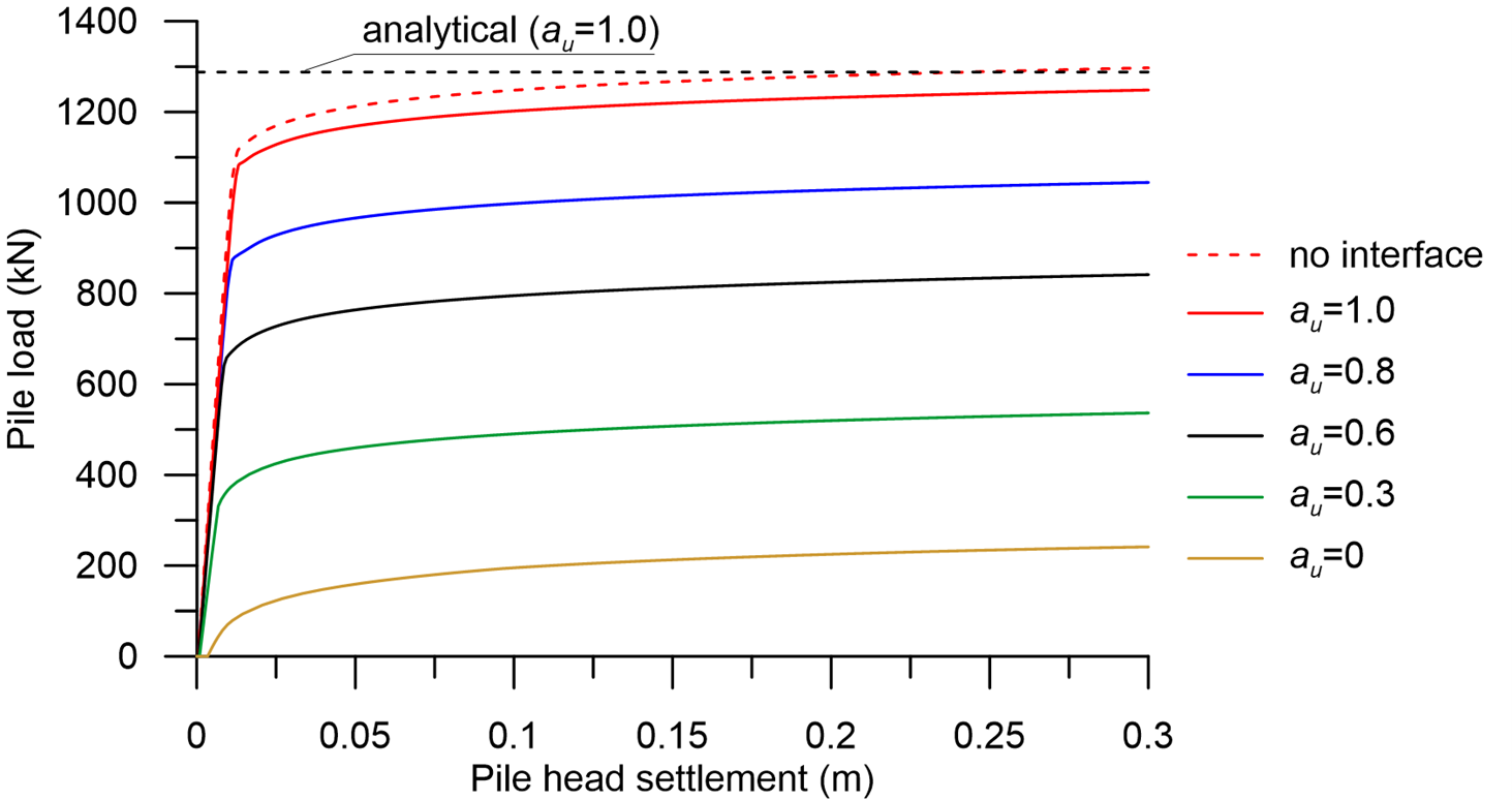
The problem here is solved parametrically, for different clay undrained Young’s modulus values Ε_u ranging from Ε_u = 1 MPa to Ε_u = 10 MPa (Figure 6.49) and different a_u values ranging from a_u = 0 to a_u = 1.0 (Figure 6.50). Additional analyses were also performed to identify the effect of separation at the soil-pile interface on the results (Figure 6.51), comparing the load-displacement curve that resulted from a model where no separation was allowed at the interface (no interface elements were employed), with the load-displacement curve that resulted from a model where a “rough” interface was considered (a_u = R_int = 1.0). The ultimate geotechnical capacity was also estimated via the α-method formulas, and analytical results are compared to the numerical ones.

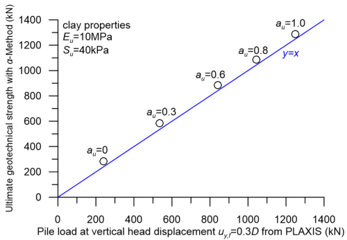
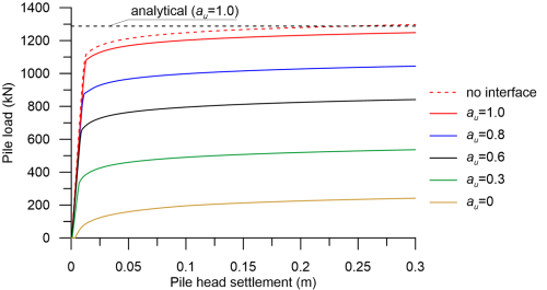
Results presented in the above figures suggest that numerical results from PLAXIS compare well with the predictions of the α-method. It is also verified that, as discussed before, that the collapse load of the pile cannot be straightforwardly identified: the load on the pile continues to increase until non-tolerable settlements develop. In the rather theoretical case where the clay layer features a very low Young’s modulus, compared to its undrained shear strength, settlements will increase to intolerable levels well before the ultimate load is applied (Figure 6.49 – Ε_u = 1 MPa). Nevertheless, for higher E_u values the sensitivity of the predicted ultimate geotechnical strength of piles in clay to the nominal pile head vertical displacement at failure u_y,f  is not particularly important (Figure 6.49).

One could argue, on the basis of the above results, that the α-method provides very reasonable estimates of the pile’s skin friction resistance under undrained conditions, therefore ICP (and other modern methods) are unnecessarily conservative. There is a caveat though. First, we have not modelled installation effects with PLAXIS, hence we did not account for soil disturbance during pile driving in our numerical model. Second, PLAXIS uses the same Coulomb model to calculate interface shear stresses, thus skin friction resistance, as the α-method. Since R_int is taken equal to a_u, skin friction estimates obtained with both methods will be very similar. Therefore the author recommends to carefully select the R_int parameter when seeking to predict the ultimate geotechnical strength with PLAXIS, ideally using methods as the ICP one for guidance.