1.8 Interpretation of CPT measurements to derive soil parameters
Except soil stratigraphy, CPT and CPTu sounding measurements can be used together with several empirical, semi-empirical as well as rigorous correlations, to determine the mechanical characteristics of soil. Soil parameters that can be derived with high-to-moderate accuracy from interpretation of CPT measurements are provided in Table 1.7. More details on the derivation of these parameters are provided in the following sections.
| Soil type | ||
|---|---|---|
| Coarse-grained (sand) | Fine-grained (clay) | |
| Relative density, Dr | ✔ | N/A |
| Earth pressure coefficient at-rest, K0 | N/R | ✔* |
| Overconsolidation ratio, OCR | N/R | ✔ |
| Sensitivity, St | N/A | ✔** |
| Undrained shear strength, Su | N/A | ✔ |
| Friction angle, φ′ | ✔ | N/R |
| Permeability (via dissipation tests) | N/R | ✔ |
| Compressibility parameters (Young’s modulus E′, coefficient of volume compressibility mv) | ✔ | ✔ |
| N/A: Not Applicable; N/R: Not Recommended | ||
| * In the author’s view, the DMT provide more reliable estimates of the earth pressure coefficient at-rest (see Chapter 1.10) | ||
| ** In the author’s view, sensitivity values obtained by means of CPT tests must be treated with caution (see Section 1.8.3 and Part 6) | ||
1.8.1 Equivalent N-SPT values
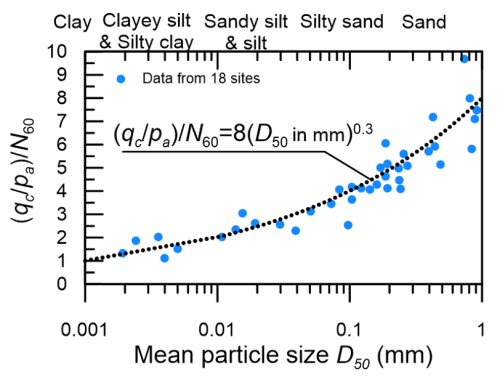
Determining equivalent N-SPT values from cone tip measurements means that we can combine CPT sounding results with the numerous empirical expressions and design methodologies that have been developed to be used together with SPT test results. Robertson and Kabal (2022) recommend using the chart presented in Figure 1.30 to estimate N60 values as a function of the cone resistance qc/pa or qt/pa, where pa = 100 kPa is the atmospheric pressure, and of the mean grain (or particle) size D50.
Alternatively, N60 values can be correlated to the cone resistance qc/pa or qt/pa while considering the SBT instead of the mean grain size, as presented in Table 1.8.
| Soil Behavior Type/Zone | Description | (qc/pa)/N60 |
|---|---|---|
| 1 | Sensitive fine-grained soils | 2.0 |
| 2 | Organic soils – Clay | 1.0 |
| 3 | Clays: Clay to silty clay | 1.5 |
| 4 | Silt mixtures: Clayey silt and silty clay | 2.0 |
| 5 | Sand mixtures: Silty sand to sandy silt | 3.0 |
| 6 | Sands: Clean sands to silty sands | 5.0 |
| 7 | Dense sand to gravelly sand | 6.0 |
| 8 | Very stiff sand to clayey sand (probably cemented) | 5.0 |
| 9 | Very stiff fine grained (heavily overconsolidated or cemented) | 1.0 |
For example, a clayey soil classified as SBT 3 and exhibiting cone resistance during penetration qt = 2 MPa has an equivalent N60 value of:
(1.15) 
1.8.2 Undrained shear strength, Su
The undrained shear strength of fine-grained soil is not a fundamental soil property, and depends on the stress level and the loading history i.e., the overconsolidation ratio OCR. The undrained shear strength can be correlated to the cone resistance by means of the following semi-empirical formula:
(1.16) 
where σz0 is the total vertical geostatic stress at the specific depth, and the cone factor Nkt ranges from 10 to 18. Equation 1.16 is analogue to the formula providing the bearing capacity of a foundation on undrained soil. Therefore, the cone factor accounts for the shape of the failure surface developing in the soil as the cone tip is being pushed downwards, and depends on the characteristics of the particular soil tested. An average value of Nkt= 14 to 16 provides acceptable, conservative results for usual cases. According to Lunne et al. (1976), Nkt can be correlated to the soil plasticity index PI (%) as:
(1.17) 
A more recent expression for estimating the cone factor Nkt has been proposed by Mayne and Peuchen (2022), who statistically analysed data from 70 clay deposits to establish a correlation between Nkt and the normalised pore pressure parameter Bq = Δu/qn :
(1.18) 
where Δu = u2 – u0 (u0 is the hydrostatic pore pressure) and qn = σt – σz0.
The undrained shear strength ratio to the geostatic vertical effective stress (Su/σ′z0) is estimated as:
(1.19) 
where

is a dimensionless expression for the cone resistance. For normally consolidated clays with OCR = 1 it is Qt = 3 to 4, thus the undrained shear strength ratio will attain a value of about Su/σ′z0 ≈ 0.22, as discussed in the Example 1.1.
An important drawback of the above expressions is that the cone factor Nkt must be assumed, determined from empirical expressions, or alternatively calibrated on the results of triaxial tests on undisturbed samples and/or in situ vane shear test data from the same site. Such data are not always available. While empirical equations such as Eq. 1.17 have some value in estimating the cone factor, they are not based on a rigorous theoretical background. An alternative method for interpreting CPTu measurements in soft clay to obtain undrained strength values, that does not require estimating a cone factor value and is based on a rigorous cavity expansion model has been proposed by Zhang et al. (2023). The undrained shear strength is calculated as:
(1.20) 
Where u2 is the pore pressure measured during the piezocone test at a certain depth, and Nu is an alternative (because Eq. 1.20 uses pore pressure instead of total vertical stress used in Eq. 1.16) cone factor, defined as:
(1.21) 
where Mcs is the inclination of the critical state line in p′–q space equal to Mcs = 6sinφcs/(3-sinφcs), that can be measured from standard triaxial compression tests. Typically, Mcs for Australian clays ranges between Mcs = 1.2 to 1.3; αE is a factor that accounts for rate effects during cone penetration, and can be taken equal to αE = 1.64 if standard CPTu penetration rates have been applied during testing; a is the half of cone tip angle. For a standard cone a = 30 deg and cota = 1.732.
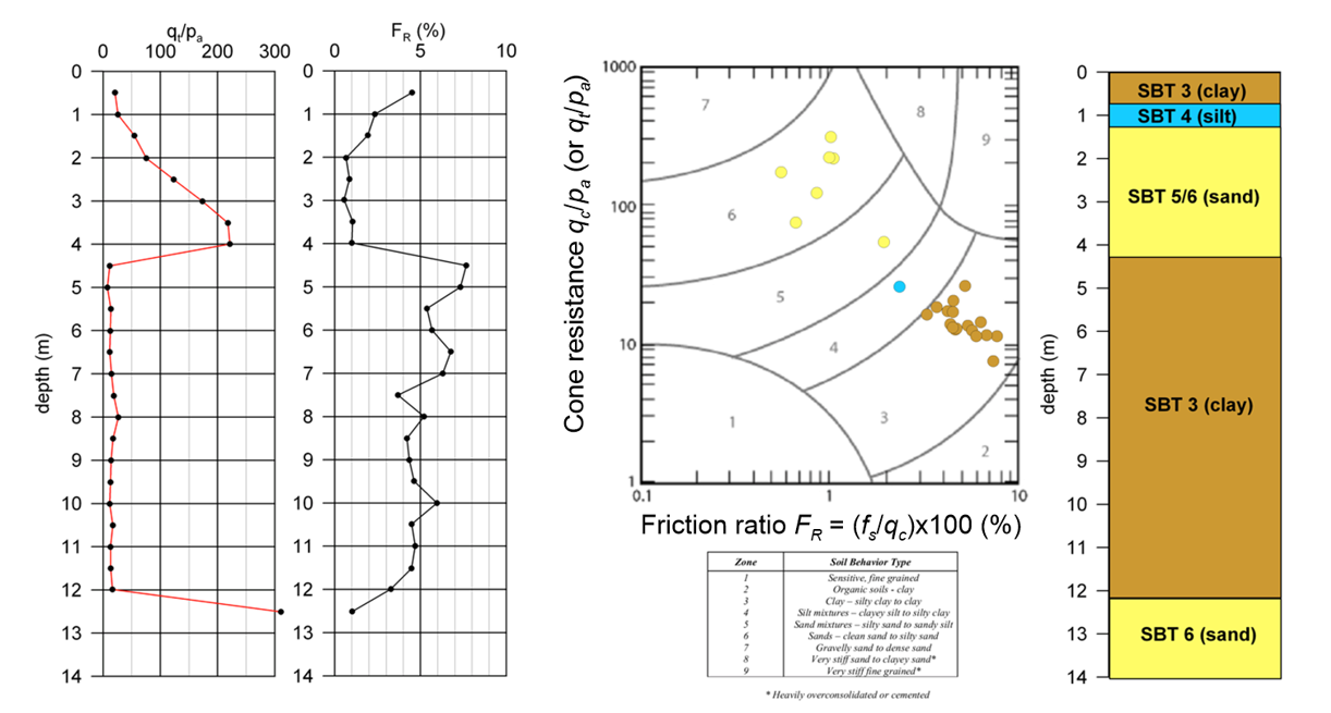
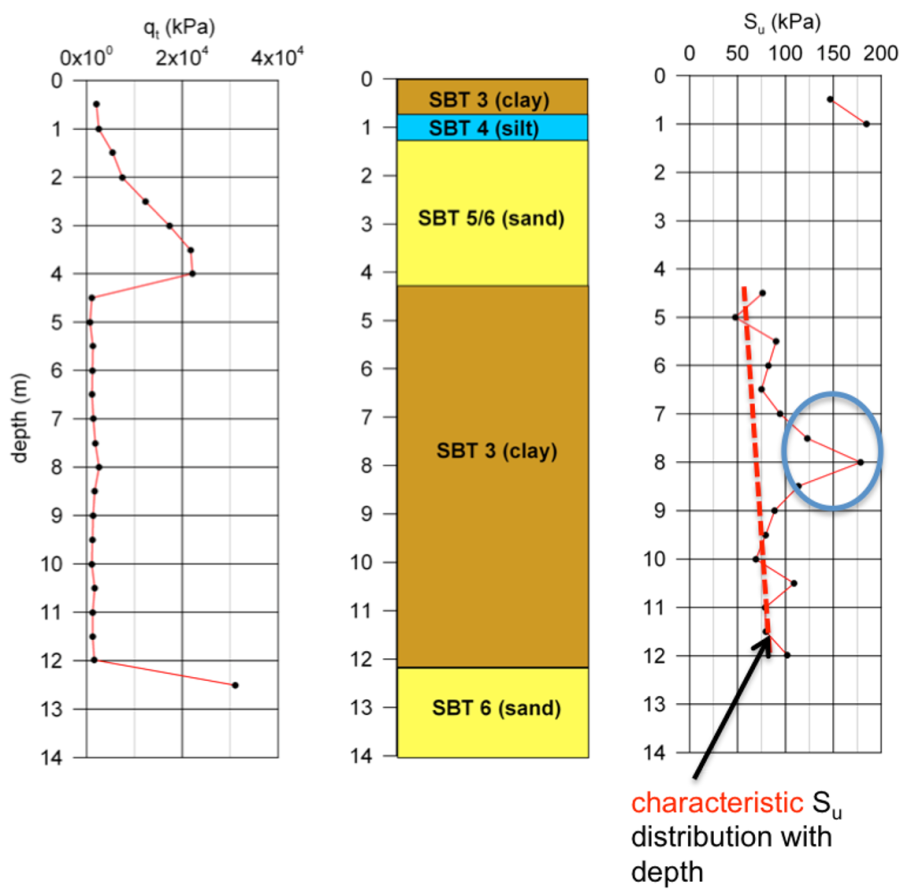
When using CPT sounding results to estimate the variation of undrained shear strength with depth, care must be taken so as to disregard any unrealistic, extreme values (Figure 1.31). Of course, undrained shear strength should not be estimated for layers expected to behave as drained, according to their Soil Behavior Type assessment.
1.8.3 Clay sensitivity, St
Clay sensitivity is defined as the ratio of the undisturbed peak undrained shear strength to the remolded undrained shear strength, at the same moisture content (Table 1.9). If disturbed, the structure of very sensitive clays will be altered and they may undergo flow, a phenomenon that may result in catastrophic mudflows.
Sensitivity values can be estimated from CPT test results as:
(1.22) 
where Fr (%) is the normalised sleeve friction resistance, defined in Eq. 1.14.
| Clay classification | Clay sensitivity, St |
|---|---|
| Insensitive | ~1.0 |
| Slightly sensitive | 1 to 2 |
| Medium sensitive | 2 to 4 |
| Very sensitive | 4 to 8 |
| Slightly quick | 8 to 16 |
| Medium quick | 16 to 32 |
| Very quick | 32 to 64 |
| Extra quick | > 64 |
For very sensitive clays, the above estimate of sensitivity should be used as a guide only, due to difficulties in accurately measuring the sleeve friction is such clays (Robertson and Kabal 2022).
1.8.4 Overconsolidation ratio, OCR and lateral earth pressure coefficient at-rest, K0
The overconsolidation ratio is commonly defined as the ratio of the maximum past vertical effective consolidation stress, σ′p over the present vertical effective stress, σ′z0. According to Robertson and Kabal (2022), OCR can be estimated from CPT test results as:
(1.23) 
where
The above Eq. 1.23 has been derived while assuming that the undrained shear strength over geostatic vertical effective stress ratio of overconsolidated (OC) clays can be correlated to the corresponding ratio for normally consolidated (NC) clays as:
(1.24)
where the exponent m is approximately equal to m = 0.8 to 0.85. This value of OCR can be also used to estimate the lateral earth pressure coefficient at-rest K0 of low plasticity clays and silts (Kulhawy and Mayne, 1990):
(1.25) 
Alternatively, the method of Zhang et al. (2023) can be used to obtain a more rigorous estimate of the overconsolidation ratio of soft clays:
(1.26) ![{\rm{OCR}} = 2{\left[ {\dfrac{{6\left( {{q_t} - {u_2}} \right)}}{{{N_u}{M_{cs}}\left( {1 + 2{K_0}} \right){{\sigma '}_{z0}}}}} \right]^{\tfrac{\lambda }{{\lambda - \kappa }}}}](https://oercollective.caul.edu.au/app/uploads/quicklatex/quicklatex.com-82bef17c194fe0a5ceea99a0db841b59_l3.png "Rendered by QuickLaTeX.com")
where K0 can be calculated as K0 = 1-sinφ′ while λ = Cc/2.3 and κ = Cr/2.3 with Cc, Cr being the compression and recompression indexes, respectively, measured from oedometer tests. Note here that κ cannot be directly related to Cr, and some recommend considering κ = 2Cr/2.3 instead.
1.8.5 Relative density Dr and friction angle φ‘ of sands
The relative density of sands is defined as:
(1.27) 
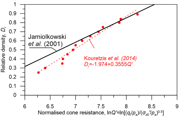
where e is the in situ void ratio, and emax, emin is the maximum and minimum void ratios corresponding to the loosest and densest state that specimens of this sand can be prepared using standarised procedures, respectively. According to Kulhawy and Mayne (1990), relative density Dr (%) of non-cemented sands can be estimated from the cone resistance as:
(1.28) 
Where Qtn is given by Eq. 1.10. Alternatively, the chart and expression presented in Figure 1.32 can be used.
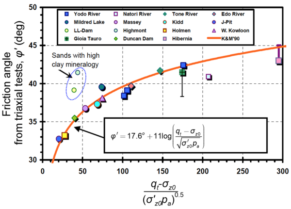
For estimating the friction angle of non-cemented sands, Mayne (2006) recommends the following expression, based on in situ and laboratory test results (Figure 1.33):
(1.29) 
1.8.6 Soil unit weight, γ
When soil samples are not available, the bulk unit weight of soil can be estimated from CPT measurements as (Robertson and Kabal 2022):
(1.30) ![\dfrac{\gamma }{{{\gamma _w}}} = \left\{ {0.27\left( {\log {F_R}} \right) + 0.36\left[ {\log \left( {\dfrac{{{q_t}}}{{{p_a}}}} \right)} \right] + 1.236} \right\}\dfrac{{{G_s}}}{{2.65}}](https://oercollective.caul.edu.au/app/uploads/quicklatex/quicklatex.com-03aad07036a77378051bc93229b250e2_l3.png "Rendered by QuickLaTeX.com")
where FR is the friction ratio (%) from Eq. 1.9; γw is the unit weight of water (10 kN/m3) and Gs is the specific gravity of soil, equal to about Gs = 2.65 for most silica-based soils.
1.8.7 Compressibility parameters E′ and mv
The drained Young’s modulus E′ of non-cemented silica sands to be used for settlement estimations (strain levels of the order of 0.1%) can be estimated from Eq. 1.31:
(1.31a) 
where
(1.31b) 
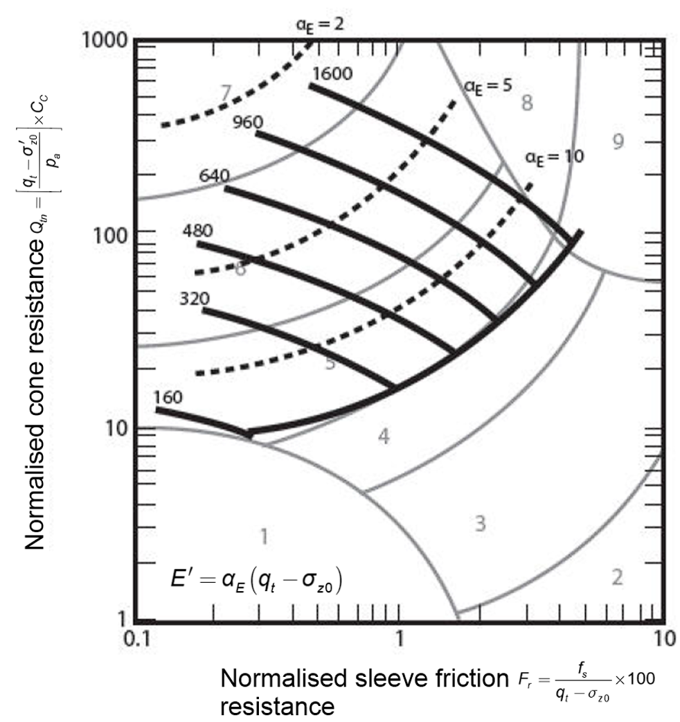
and Ic is the Soil Behaviour Type index, calculated according to Eq. 1.13. The parameter αΕ can be estimated alternatively from Figure 1.34.
![Graph showing αE values for sand-like materials as function of the normalised cone resistance [(qt-σ'z0)/pa]Cc and the normalised sleeve friction resistance Fr](https://oercollective.caul.edu.au/app/uploads/sites/143/2024/12/1.34-HR-e1743560565182.png)
The coefficient of volume compressibility mv of fine-grained soils, which is correlated to their Young’s modulus and Poisson’s ratio by means of theory of elasticity formulas (see Part 4), can be evaluated as:
(1.32) 
where:
(1.33a) 
(1.33b) 
Note that the above expressions are valid when the Soil Behaviour Type index is Ic > 2.2, which corresponds to fine-grained soils.
