Example 4.7

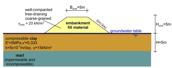
The approach embankment (transition from embankment to bridge) of the figure below is going to be founded on a compressible clay of thickness H = 5 m. Estimate the necessary time that the embankment should be left to settle before constructing the pavement layer, for its post-construction settlement to be less than 10 mm. Assume that the time required for the construction of the embankment is negligible.

Answer:

The pressure applied on the subsoil from the embankment is non-uniform and its width, at least in the area of maximum embankment height, is comparable to the thickness of the compressible layer. The above suggest that the two-dimensional plane-strain consolidation problem must be simulated. Note that a closed-formed solution is not available for two-dimensional consolidation problems, and numerical methods (not necessarily the finite element method) are used to determine the excess pore water pressure and settlement evolution with time.

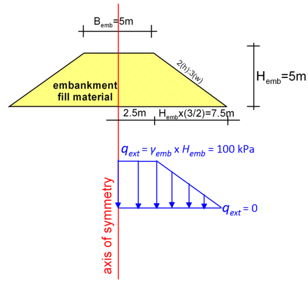
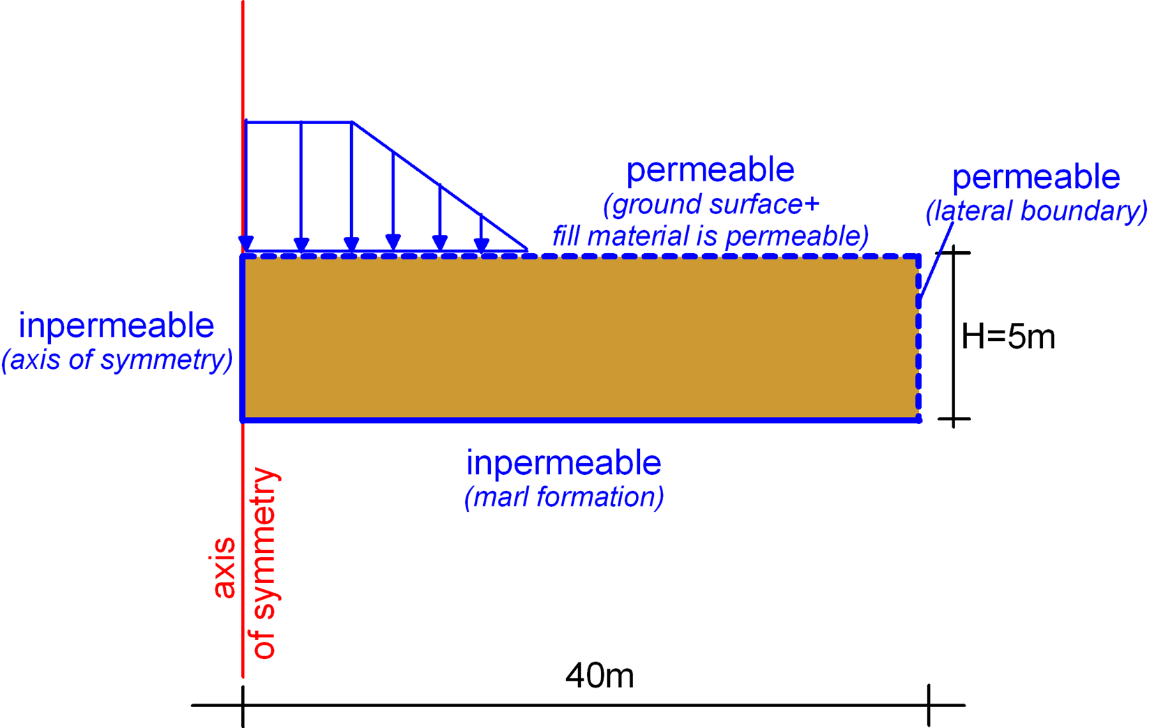
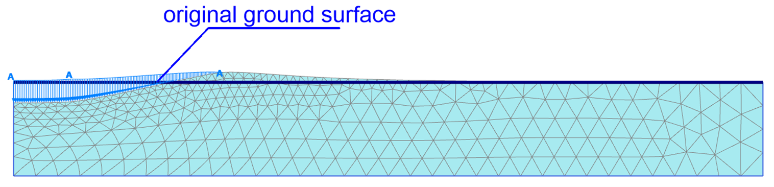
The problem is symmetric, with the axis of the embankment being the plane of symmetry. Given that we are not interested in the embankment stability conditions, instead of simulating the embankment itself, we will replace it with a distributed pressure (Figure 4.49). However, we can most certainly model the actual fill, as a separate geometry cluster comprising permeable (free-draining) linear elastic material with unit weight γ_emb = 20 kN/m³. To obtain results similar to those with the model where the embankment is simulated as a pressure, we must assign very low stiffness and very high permeability to the material representing the fill, to approximate free dissipation of excess pore pressures from the body of the embankment, and flexible loading. Nevertheless, the stiffness of the fill material and its permeability will not have a particularly important effect on predicted settlements for the problem at hand.

“Standard fixities” will be applied as displacement boundary conditions. The marl formation is not simulated, and will be replaced by fixed displacements at the bottom of the clay layer, as in Example 4.6.

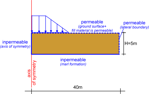
As far as drainage boundary conditions are concerned: The left lateral boundary is an axis of symmetry, thus no flow should be allowed, and an impermeable boundary should be considered. The right lateral boundary, which should be placed in sufficient distance from the embankment toe equal to about 3 times the half-width of the embankment, should be permeable, as the clay layer extents “infinitely” along the horizontal direction. This rule-of-thumb for determining the distance of the lateral boundaries from the area of interest must always be used with caution, and the sensitivity of the analysis model to the boundary conditions must always be checked by means of parametric analysis. Permeable boundary conditions must be applied to the ground surface too. The ground surface must be permeable along its full extent, as the embankment is constructed of free-draining material (Figure 4.50).

The undrained (A) linear elastic model is used to simulate clay behavior under the applied pressure, as in Example 4.6, allowing for the calculation of (excess) pore water pressures for plastic stages too. Soil compressibility is defined in terms of effective parameters i.e. the drained Young’s modulus E′ and Poisson’s ratio v′ as used as input, but the undrained stiffness parameters are calculated internally by PLAXIS. The permeability of the clay, k is also entered as a material parameter. Two distributed pressures are applied, a uniform and a triangular one, with the values and the widths presented in Figure 4.49.

The analysis consists of three stages:

• Step 1: Initial phase. The geostatic stresses and hydrostatic pore water pressures before the application of the external pressure are initialised with the “K0-procedure”. Drainage boundary conditions and the water table level are defined, as in Figure 4.50.
• Step 2: Sudden application of the loading. A “Plastic” step is introduced, where the external pressure is instantaneously applied on the ground surface i.e., the time interval of this step is 0.0 days. This corresponds to instantaneous construction of the fill.
• Step 3: Consolidation. A “Consolidation” step follows the previous plastic step, where the analysis will continue until the degree of consolidation reaches 99%, and excess pore pressures developed during Step 2 will have practically fully dissipated. The loading option “Degree of Consolidation” is selected for that. “Reset displacements to zero” should not be active, so that the immediate settlement, which in that case is expected to be a considerable portion of total settlement, will be co-estimated.

Note that when the “Degree of Consolidation” option is used to define the end of the simulation, care must be taken to ensure that excess pore pressures in the area of interest (below the embankment) have dissipated and settlement has indeed stabilised. The reason for that is that PLAXIS calculates the average degree of consolidation across the simulated compressible layer, and significant pore pressure gradients may remain in the area of interest, even when the average degree of consolidation across the 40m-wide clay layer approaches U = 100%. This reiterates the importance of carefully selecting the distance of the boundaries from the area of interest, instead of following rules-of-thumb without judgment.

In this particular example we assume for simplicity that the fill is placed “instantaneously”. However, we can actually model staged construction of the fill in PLAXIS. This can be achieved by replacing the “Plastic” step 2 with a “Consolidation” step, of duration equal to the time required for the construction of the fill. In that case the pressure will not be applied instantaneously, but instead will be ramped-up to its final value, which will be reached at the end of the step. Assuming that the pressure increases linearly with time during the construction period will provide a more accurate estimate of pore pressures that will develop in soil in situ, which may be important if stability of the embankment during construction is assessed. Finally note that time has no physical meaning in “Plastic” steps, and is only used for presentation of analysis results. Even if a time value is entered as input for a plastic step, the entire pressure will be applied instantaneously in the beginning of the step, and held constant thereafter.

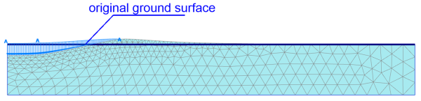
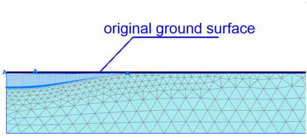
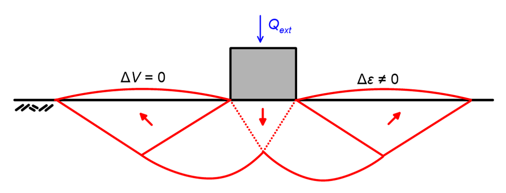
The deformed mesh at the area of the embankment at the end of Step 2, immediately after the application of the pressure, is presented in Figure 4.51. Notice that the immediate settlement due to the construction of the embankment is not negligible, and it reaches about ρ_e = 22 mm. As discussed in Chapter 4.4 soil deformation under short-term undrained conditions takes place without volume change (Figure 4.9), and soil heaves around the loaded area (Figure 4.51).

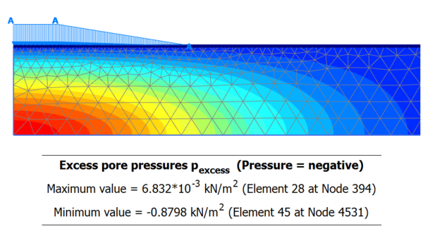
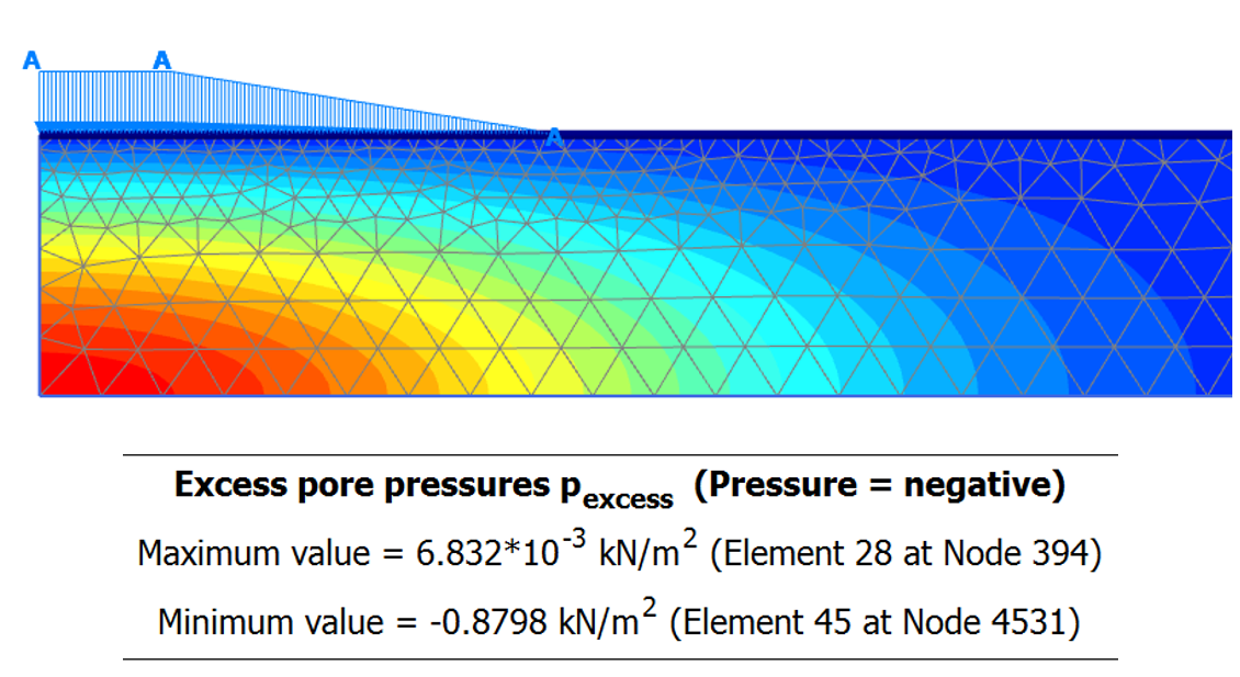
At the end of Step 3, when the average degree of consolidation has reached U = 99%, excess pore pressures are practically reduced to zero, with its maximum value being Δu = 0.88 kPa below the axis of the embankment and near the impermeable marl layer boundary (Figure 4.52a). Total settlement of the soil surface has reached ρ = ρ_e + ρ_pc = 70 mm, and soil heave is now negligible, as volume changes in long-term drained loading conditions.

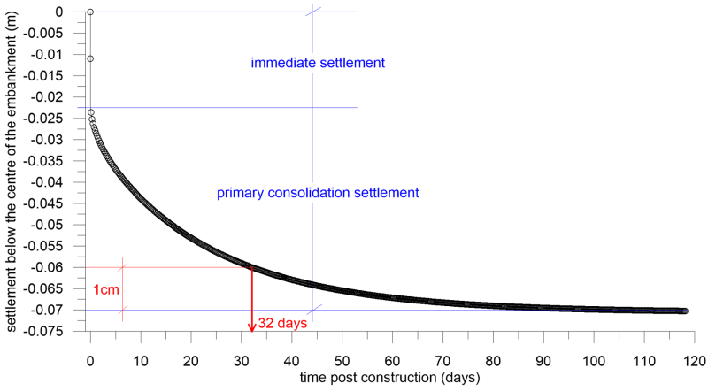
The evolution of settlement with time is presented in Figure 4.53. Notice that part of settlement develops instantaneously, and is the immediate settlement calculated from Step 2, while primary consolidation settlement evolves with time. To find the necessary time that the embankment must be left to settle before constructing the pavement layers, we need to find from the settlement curve in Figure 4.53 the time when settlement reaches the final value of settlement minus the allowable post-construction settlement 70 mm – 10 mm = 60 mm (about 32 days).