Example 3.2
Numerical estimation of stresses below a ring-type foundation
Solve Example 3.1 numerically with PLAXIS, and compare the results to the analytical solution.
Answer:
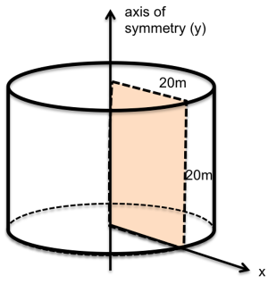
The problem is simulated in PLAXIS as axisymmetric, considering soil to be a linear elastic material. To obtain a first approximation of the necessary thickness of the soil mass that must be simulated to get accurate results, one may consider Eq. 3.16 suggesting that the influence depth of a circularly loaded area is equal to four times the radius of the footing. In this case where rexternal = 5 m, we can assume that additional stresses due to the external loading will have attenuated to 10% of the stress applied on the foundation surface at a depth of 20 m, and start our simulation by modelling an area of dimensions 20 m x 20 m (Figure 3.16).
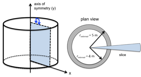
Since the problem is axisymmetric, we are simulating a “slice” of the soil, of thickness equal to 1 rad, as shown in Figure 3.17 below. The axis of symmetry of the numerical model will be the axis of symmetry of the ring foundation, passing through its centre.
The linear elastic material model is used to model soil response to the external loading. Since we are interested only in stress increments due to the external loading, the unit weight of the soil should be set equal to zero, so that geostatic stresses will not be calculated. As expected from theory (Chapter 3.5 and Eq. 3.13), the compressibility parameters that will be used as input for the linear elastic material model i.e., the Young’s modulus and the Poisson’s ratio should not affect the predicted magnitude and distribution of stresses. However, considering for example an unrealistically low value for the Young’s modulus will result in extreme soil settlements, and perhaps affect the results due to numerical issues.
Footing pressure is applied as a vertical distributed pressure along the area of the ring footing (Figure 3.17). The footing itself is not simulated, and stress is applied directly on the soil surface, so as to be in line with the “flexible” foundation assumption inherited in the analytical formulas, as mentioned in Chapter 3.7.
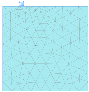
A “coarse” mesh is defined after the application of the pressure (Figure 3.18), which should be adequate for the simulation of the elastic problem at hand, and standard fixities are applied at the boundaries of the grid. When an axisymmetric model is built in PLAXIS, standard fixities will apply the necessary zero in-plane displacement and zero in-plane rotation along the axis of symmetry defined by the center of the footing.
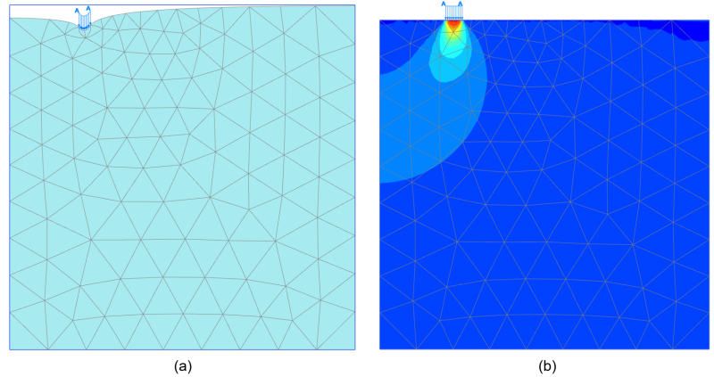
The analysis is run in a single “plastic” step, whereas the initial “K0-procedure” step should result in zero geostatic stresses for this model, as the unit weight of the soil was assumed equal to zero. A plot of the resulting deformed mesh is presented in Figure 3.19a, and a plot of the vertical stress contours in Figure 3.19b.
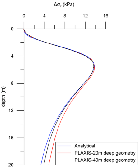
Results are compared to the analytical solution in Figure 3.20, by plotting the additional vertical stress distribution with depth along the axis of the footing. Notice that the basic PLAXIS analysis (red line) compares well with analytical results (blue line), in the area of interest, where the maximum stress develops. However, the two solutions diverge at larger depths. This is expected, as the analytical solution has been derived while considering an elastic half-space. This assumption is not satisfied near the bottom boundary of the finite element mesh, where displacements are fixed along both the horizontal and vertical directions. An additional analysis performed for a 40-m deep model (black line) results in much better agreement with the analytical solution along the top 20 m of the axis of symmetry.
