Example 1.1
Establishing a geotechnical model for the geotechnical design of a bridge foundation
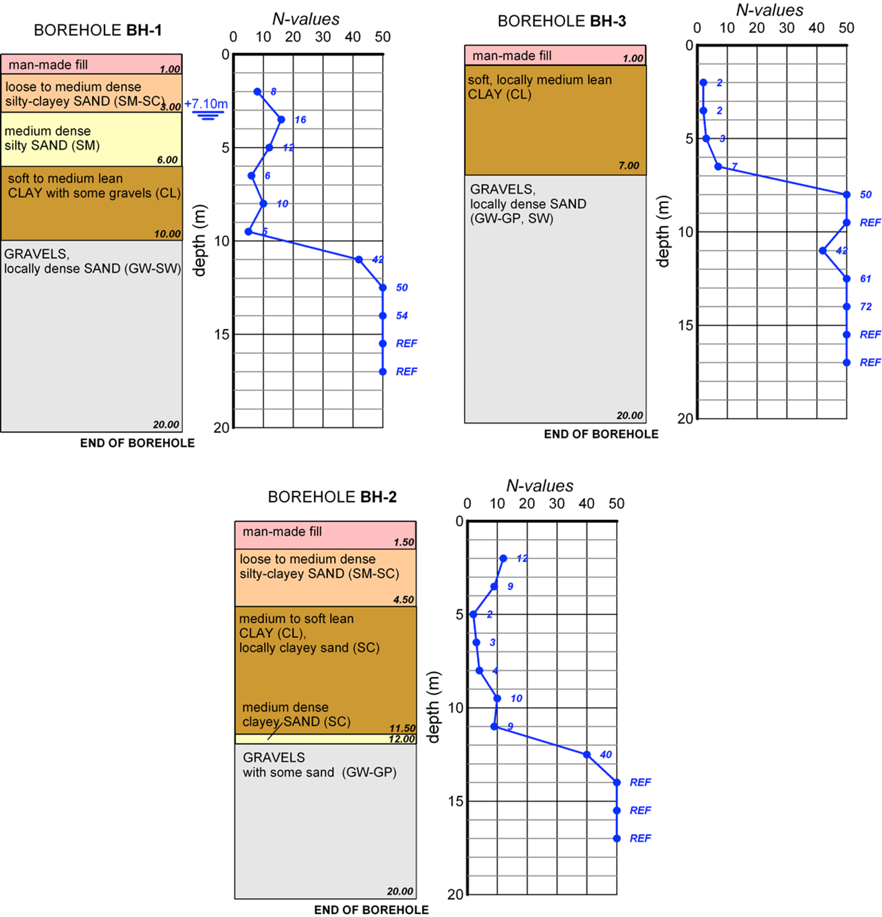
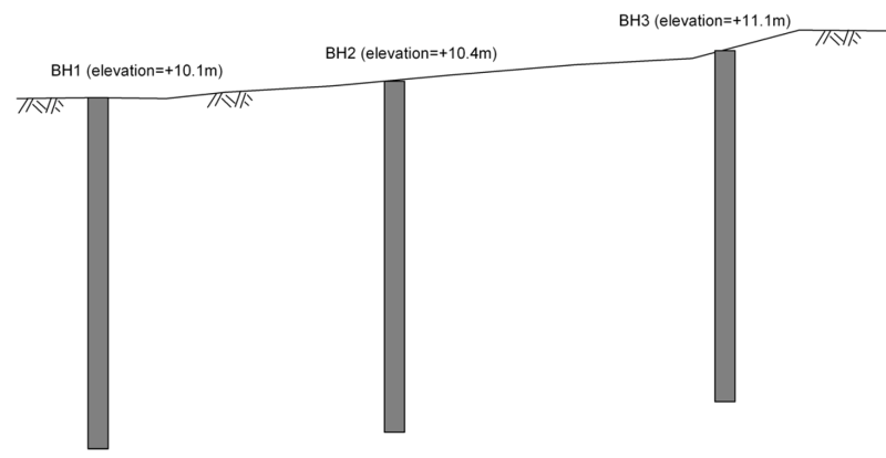
For the geotechnical design of a new bridge, 3 boreholes (BH-1, BH-2 and BH-3) were drilled, spaced 15 m apart. SPT tests have been performed, while a piezometer was installed in BH-1, measuring the absolute groundwater table level at +7.10 m. Create a simplified geotechnical profile of the site, and determine the strength and compressibility parameters of each geotechnical layer; in other words, propose a geotechnical model of the area.
Answer:
Trying to unify findings from the borehole logs into layers that will exhibit similar geotechnical behavior includes identifying the number of layers required to sufficiently describe the subsoil conditions, their geotechnical description, and their extent both vertically and laterally.
In this particular case, one may define the geotechnical layers and their geometry, while considering the following:
- The top artificial fill layer, of thickness 1.0 m to 1.5 m, may have to be removed or treated before the construction of the foundation e.g., replaced with an improvement layer. Foundation of structures on uncontrolled (existing) fills is generally not recommended, due to their variable composition.
- Very thin layers, such as the medium dense clayey sand layer found in borehole BH-2 from 11.5 to 12.0 m can be effectively ignored, as they will not alter the overall geotechnical response of the foundation.
- Layers of similar classification according to USCS and similar degree of consistency, as the loose-to-medium dense silty-clayey sand found in boreholes BH-1 and BH-2 can be unified, while adopting a rather conservative approach to define their shear strength and compressibility parameters.
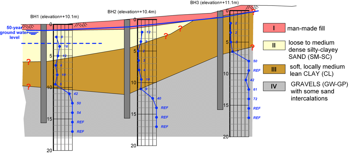
- When we are not sure about the geometry of a layer, use question marks (?)
Following the above guidelines, and considering the design groundwater level at least 2 m above the measured one to account for fluctuations during the lifetime of the project, we come up with the geotechnical layers and their possible geometry presented in the cross-section below (Figure 1.18).
For the derivation of design geotechnical parameters, the SPT blow counts are used together with empirical correlations, and of course engineering judgement. Creating (corrected or uncorrected) SPT plots with depth, separately for each geotechnical layer, is very useful when it comes to defining an average and a “characteristic” SPT value for this layer, to be used with the empirical correlations. This approach is demonstrated in the following two figures, while more on the determination of characteristic values of soil parameters are provided in Part 5 and AS5100.3.
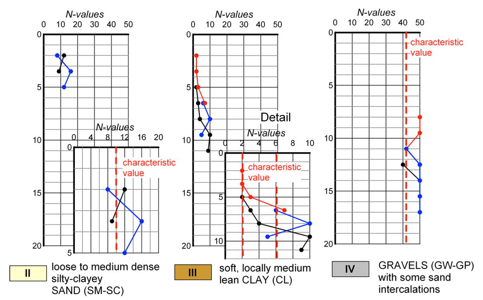
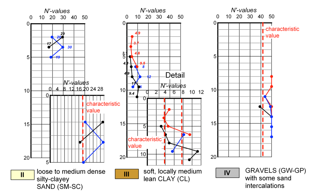
For correcting SPT blow counts to overburden stress, it was assumed for simplicity that the unit weight of all soil layers is equal to γ = 18 kN/m3 and, for the calculation of the distribution of geostatic vertical effective stress with depth σ′z0, that the groundwater table at the time when boreholes were drilled was at the ground surface. Notice that, if SPT measurements suggest so, we may consider a different characteristic N value for the same layer, but for different depths, as for layer III.
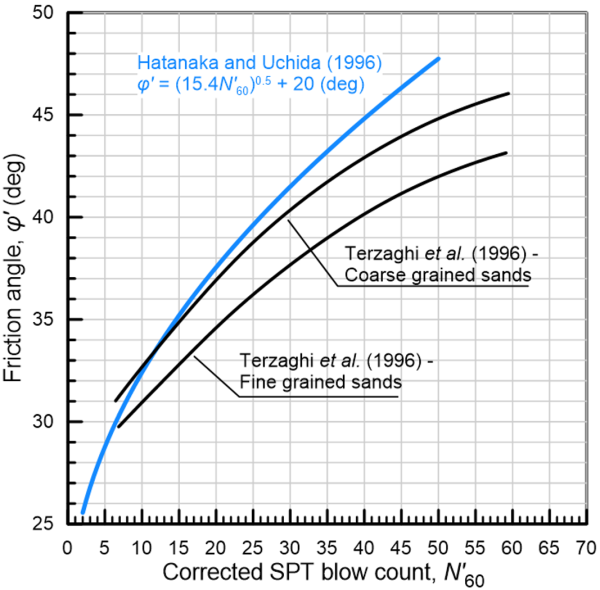
Given the characteristic values from the above graphs, which correspond to a reasonable lower bound of SPT blow counts, we can estimate the friction angle φ′ of the coarse-grained geotechnical layers II and IV from Figure 1.16. Selection of this characteristic value (or reasonable lower bound) depends on the amount of available information: If a large number of SPT measurements are available, it is reasonable to select a characteristic value close to the mean SPT value. On the other hand, if only a handful of measurements are available (refer to Unit II in Figures 1.19 and 1.20), it is prudent to select a characteristic value close to the lower bound of measurements.
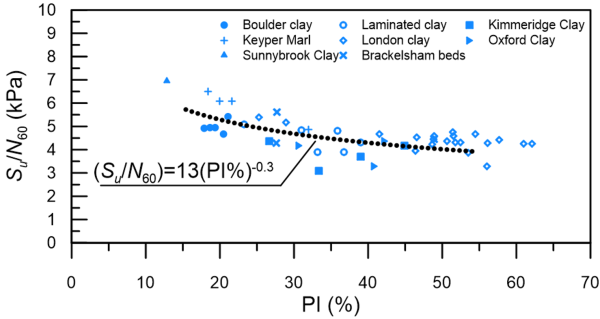
The undrained shear strength Su of the fine-grained geotechnical layer III can be estimated from Figure 1.17, while assuming that this low-plasticity clay has an average plasticity index PI = 20%, in the absence of laboratory test results. While doing so we need to keep in mind that the undrained shear strength is not a soil property, but function of both the water content and of the effective stress level (for normally consolidated clays it is Su/σ′z0 ≈ 0.22). It is therefore reasonable to consider that the undrained strength Su will increase with depth.
Furthermore, the Young’s modulus Εs of all three layers defined here is estimated from Table 1.5, from the expression for sand for layer II, the expression for gravelly sand for layer IV, and the expression for clay with PI > 15% for layer III. Note that blow counts must be converted from N70 to N55 for 55% hammer efficiency in order to be used with the expressions of Table 1.5, as:

Considering the dynamic nature of the SPT test, it is reasonable to consider that Young’s moduli Es interpreted from SPT tests in fine-grained soils are undrained moduli (Eu), while deformation moduli interpreted from SPT tests in coarse-grained soil are drained moduli (E′). Results are presented in a summary table below, together with the characteristic N values considered, a table that is included in every geotechnical investigation report.
| Geotechnical Layer | Uncorrected characteristic SPT value, N | Corrected characteristic SPT value, N′ | Effective cohesion, c′
(kPa) |
Friction angle, φ′ (deg | Undrained shear strength, Su (kPa) | Young’s modulus, Eu or E′ (MPa) | Behaviour under short term loads |
|---|---|---|---|---|---|---|---|
| II | 10 | 18 | – | 31 | – | 21 | Drained |
| III (above -8m) | 2 | 4 | 2* | 26* | 12 | 2 | Undrained |
| III (below -8m) | 6 | 8 | 2* | 26* | 36 | 6 | Undrained |
| IV | 40 | 40 | – | 43 | – | 45 | Drained |
* Estimated from laboratory triaxial tests on undisturbed samples
There are a number of empirical relations in the literature that we can base our soil parameter estimation on. Usually not just one, but rather two or more are considered for each parameter in everyday engineering practice. This provides us a range rather than a single value for each parameter, and accounts for uncertainties inherited in the use of such approximate expressions. Complementing laboratory test results with these findings will lead to more comprehensive evaluation of the response of the various geotechnical layers.
