6.27 Numerical beam-on-nonlinear Winkler spring methods for the analysis of piles subjected to lateral loading

George Kouretzis

6.27 Numerical beam-on-nonlinear Winkler spring methods for the analysis of piles subjected to lateral loading

One important drawback of analytical methods, such as that of Broms, is the assumption of uniform soil conditions along the length of the pile. Since piles embedded in uniform soil are probably the exception rather than the rule, numerical methods are now being used extensively in practice for the analysis of piles subjected to lateral loading. Even relatively simple methods, such as the one described in the following, are not limited to uniform conditions (or to pile slenderness larger than the critical, as discussed earlier), and can account for multiple soil layers of varying thickness.

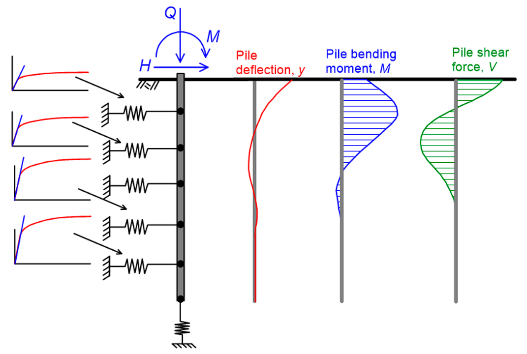
Since lateral loading of a pile is neither an axisymmetric nor a plane strain problem, two-dimensional finite element codes such as PLAXIS 2D cannot be used to model lateral loading of the soil-pile system. Instead, we use beam-on-nonlinear Winkler spring models (see Figure 6.91) where the pile is modelled as one-dimensional beam, and the soil surrounding the pile is replaced with non-linear springs, which provide the reaction on the pile p as function of its deflection y at any depth. External loads are applied on the head of the pile. While closed form solutions cannot be obtained for this problem if the p–y relationship is non-linear, we can use the Finite Element Method to discretise the pile into a finite number of beam elements, and attach spring elements at the beam elements’ nodes. Multilayered soil profiles can model in this way, by considering different p–y relationships for different spring elements. Various commercial codes based on this concept are available in the market, and referring in detail to them is not within the scope of this chapter.

Pivotal to the successful analysis of piles with this method is the selection of appropriate p–y relationships or curves, representative of the soil conditions, of the pile’s geometry and of the type of loading, and the use of realistic input parameters for these expressions. A collection of widely-used mathematical expressions that provide p–y relationships for different soil conditions is presented in the following sections, in the form of step-by-step workflows. Note that the presentation is limited to curves applicable to static, monotonic loading. For cyclic loads featuring a significant number of loading cycles, as the case of offshore platforms subjected to wave loads, the interested reader may refer to Reese and van Impe (2001).

6.27.1 p-y curves for piles embedded in soft clay, in the presence of free water

Step 1:

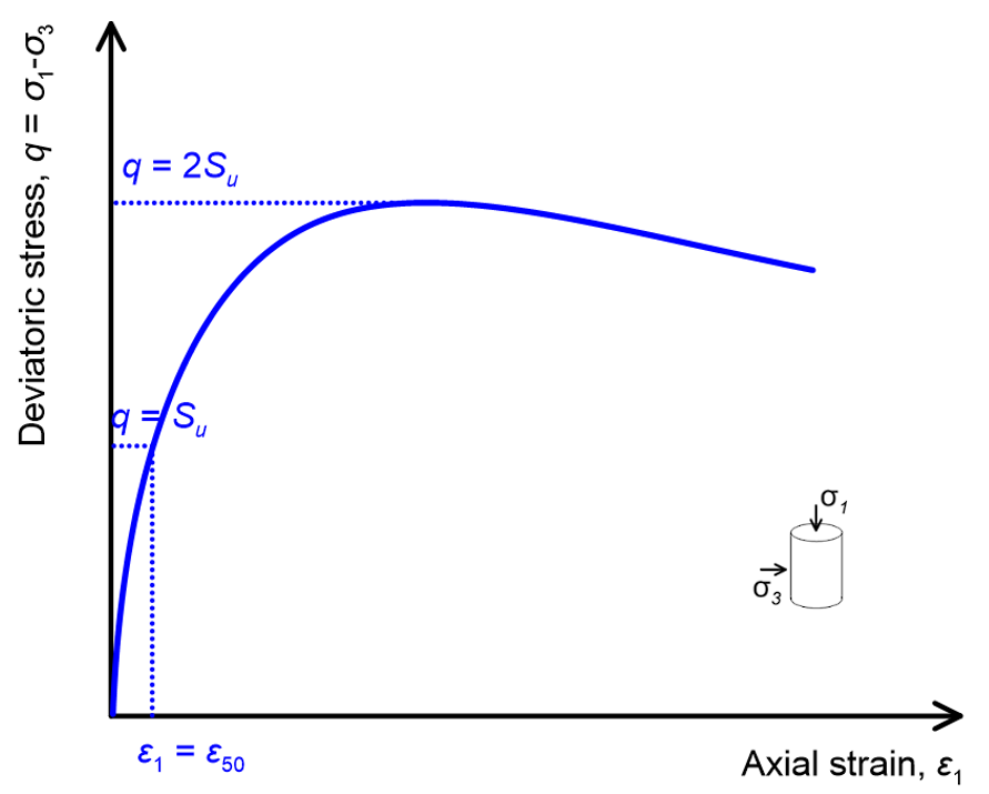
Estimate the undrained shear strength of the clay S_u, and the characteristic strain ε₅₀, which is the strain that develops in a clay sample during an undrained triaxial compression test when the deviatoric stress q on the sample becomes equal to q = σ₁–σ₃ = S_u i.e., is half the deviatoric stress at failure (Figure 6.111). If triaxial laboratory tests are not available e.g., when S_uis estimated from in situ tests, one can use the typical values listed in Table 6.17. Keep in mind that overconsolidated clays exhibit more brittle behaviour, and will fail at lower strain levels.

**Table 6.17.** Typical ε₅₀ values for soft-to-hard clays (after Peck *et al.* 1974).
Clay consistency	Undrained shear strength	ε₅₀
Soft-to-firm	S_u< 50 kPa	0.020
Firm-to-stiff	50 < S_u< 100 kPa	0.010 to 0.007
Stiff-to-hard	100 < S_u< 200 kPa	0.007 to 0.005
Hard-to-very hard	200 < S_u< 400 kPa	0.004

Deviatoric stress-axial strain plot obtained from a triaxial test on a soil sample. The maximum deviatoric stress that develops is denoted as q = 2Su. The intersection of a horizontal line at q = Su and the stress-strain plot provides the strain ε1=ε50. — Figure 6.111. Definition of the characteristic strain *ε₅₀*.

Step 2:

Compute the ultimate soil reaction per unit length of the pile as the minimum of two values:

(6.129) ${p_f} = \min \left\{ {\begin{array}{*{20}{c}}{\left( {3 + \dfrac{{\gamma '}}{{{S_u}}}z + \dfrac{J}{D}z} \right){S_u}D}\\{9{S_u}D}\end{array}} \right\}$

where γ′ = γ – γ_w is the average submerged unit weight from the ground surface to the depth z where the p-y curve is estimated; J = 0.5 for soft clays or J = 0.25 for medium-to-firm clays (Matlock, 1970). The second term of Eq. 6.129 corresponds to the ultimate soil reaction developing on a smooth rigid pile in undrained perfectly-plastic soil, mentioned earlier in Chapter 6.24.

Step 3:

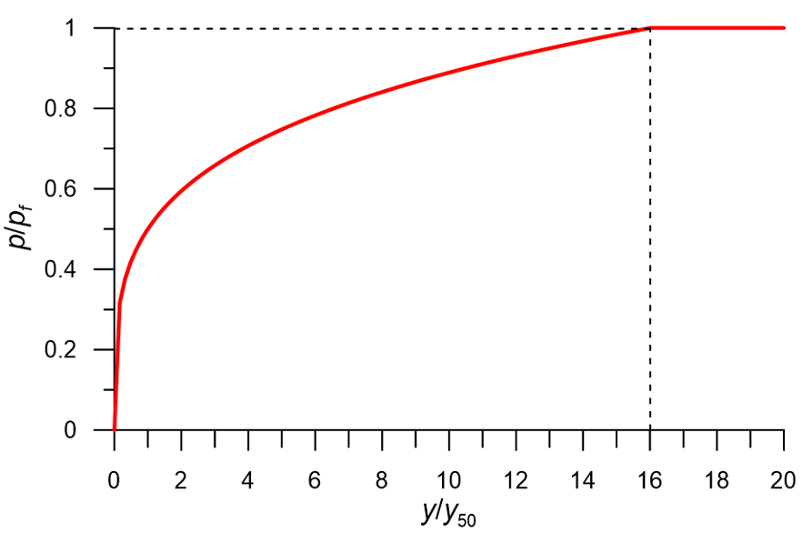
Compute the deflection of the pile y₅₀ at one-half the ultimate soil reaction p = 0.5p_f :

(6.130) ${y_{50}} = 2.5\varepsilon {}_{50}D$

Step 4:

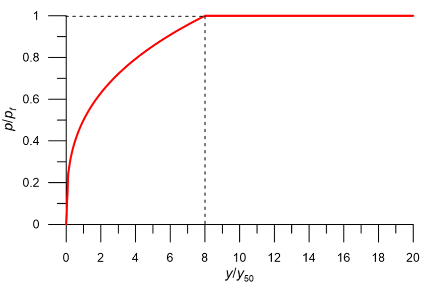
All the input parameters of the p-y curve have now been determined:

(6.131a) $p = 0.5{p_f}{\left( {\dfrac{y}{{{y_{50}}}}} \right)^{\tfrac{1}{3}}}{\rm{ \:for\: }}y < 8{y_{50}}$

(6.131b) $p = {p_f}{\rm{\:for\: }}y \ge 8{y_{50}}$

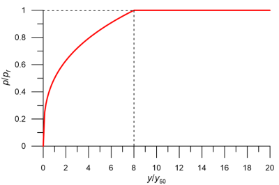
The shape of the p–y curve is depicted in Figure 6.112.

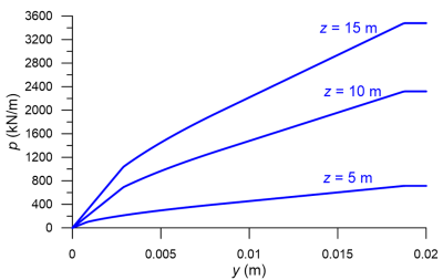
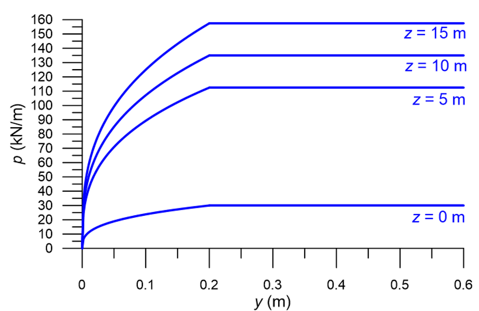
Variation of the dimensionless reaction on the pile p/pf with normalised deflection y/y50. The dimensionless reaction reaches its maximum value p/pf = 1 when y/y50 = 8 and remains constant as deflection increases further. — Figure 6.112. Shape of static *p-y* for a pile embedded in soft clay, in the presence of free water according to Matlock (1970).

For example, consider a 15-m long pile with diameter D = 0.5 m, driven in soft clay with undrained shear strength increasing with depth, z as S_u= 20+z (kPa). The submerged unit weight of the clay is taken equal to γ′ = 6 kN/m³, and it is further assumed that J = 0.5 and ε₅₀= 0.02. Substituting in Eqs. 6.129 and 6.130 yields:

(6.132) ${p_f} = \min \left\{ {\begin{array}{*{20}{c}}{\left( {3 + \dfrac{6}{{20 + z}}z + \dfrac{{0.5}}{{0.5}}z} \right)\left( {20 + z} \right)0.5}\\{9\left( {20 + z} \right)0.5}\end{array}} \right\}{\rm{ }}\dfrac{{{\rm{kN}}}}{{\rm{m}}}$

and

(6.133) ${y_{50}} = 2.5\varepsilon {}_{50}D = 0.025{\rm{\: m}}$

Variation of the ultimate soil reaction per unit length of the pile with depth z is given in Eq. 6.132. Indicatively, for z = 0:

(6.134) ${p_f} = \min \left\{ {\begin{array}{*{20}{c}}{30}\\{90}\end{array}} \right\}{\rm{ }}\dfrac{{{\rm{kN}}}}{{\rm{m}}}$

and the p-y curve is described by the function:

(6.135a) $p = 15{\left( {\dfrac{y}{{0.025}}} \right)^{\tfrac{1}{3}}}{\rm{ }}\dfrac{{{\rm{kN}}}}{{\rm{m}}}{\rm{ \:for\: }}y < 0.2{\rm{ m}}$

(6.135b) $p = 30{\rm{ }}\dfrac{{{\rm{kN}}}}{{\rm{m}}}{\rm{ \: for \:}}y \ge 8{y_{50}}$

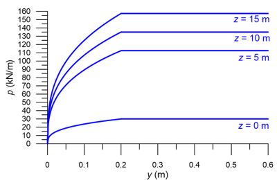
p-y curves for different depths along the length of the pile are illustrated in Figure 6.113. Notice that the ultimate soil reaction p_f increases with depth, but not the lateral pile movement necessary to mobilise it, as the latter depends only on the characteristic strain ε₅₀ and on the pile’s diameter.

Variation of reaction p with pile deflection y, for different depths z, measured from the soil surface. The ultimate reaction increases as z increases, but the deflection required to mobilise the ultimate reaction is independent of z. — Figure 6.113. Indicative *p-y* curves along a 15-m pile embedded in soft clay in the presence of free water.

6.27.2 p-y curves for piles embedded in stiff clay, in the presence of free water

Step 1:

Estimate the undrained shear strength of the clay layer S_u at the depth z (measured from the soil surface) where the curve is determined, and the average undrained shear strength over the depth z, S_u,aver.

Step 2:

Compute the ultimate soil reaction per unit length of the pile as the minimum of two values:

(6.136) ${p_f} = \min \left\{ {\begin{array}{*{20}{c}}{2{S_{u,aver}}D + \gamma 'Dz + 2.83{S_{u,aver}}Dz}\\{11{S_u}D}\end{array}} \right\}$

where γ′ is the average submerged unit weight from the ground surface to the depth z, defined above. The second term of Eq. 6.136 corresponds to the ultimate soil reaction developing on a rough rigid pile in undrained perfectly-plastic soil, as discussed earlier.

Step 3:

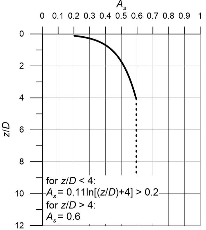
Estimate the factor A_sfrom the expressions presented in Figure 6.114, as function of z where the curve is determined. The provided expressions are for static, monotonic loads.

Graph presenting the variation of the parameter As with dimensionless depth z/D. For z/D < 4 As is calculated as As = 0.11ln[(z/D)+4] > 0.2 and for z/D > 4 As is constant As = 0.6. — Figure 6.114. Variation of factor *A_s* with normalised depth *z/D*; Piles in clay.

Step 4:

Establish the initial straight-line part of the p-y curve, referred to as linear (1) in Figure 6.115:

(6.137) $p = {k_s}zy$

The inclination of its slope k_s is provided in the Table 6.18 below.

Table 6.18. Slope of the initial straight line part of the p-y curve for piles embedded in stiff, clay under the presence of free water (Reese and van Impe 2001).

Average undrained shear strength to depth z where the p–y curve is estimated	k_s (static, kN/m³)
S_u= 50 to 100 kPa	135000
S_u= 100 to 200 kPa	270000
S_u= 300 to 400 kPa	540000

Graph presenting the different segments of a p-y curve. The segment linear (1) provides the initial slope while the segment parabolic (1) describes the p-y curve up to deflection Asy50. The segment parabolic (2) describes the p-y curve from deflection Asy50 to deflection 6Asy50. The segment linear (3) describes the p-y curve from deflection 6Asy50 to deflection 18Asy50. The segment linear (4) describes the p-y curve for deflection larger than 18Asy50. — Figure 6.115. Segments of static *p-y* curve for a pile embedded in stiff clay, in the presence of free water. Monotonic static load case (after Reese et al. 1975).

Step 5:

Compute y₅₀=ε₅₀D. In the absence of undrained triaxial compression laboratory tests, one may use the typical values of ε₅₀ provided in Table 6.17 above.

Step 6:

Establish the first parabolic part of the p-y curve, named parabolic(1) in Figure 6.115, using the following Eq. 6.138. It defines the part of the parabolic curve from the intersection with the initial straight line up to a pile lateral deflection equal to A_sy₅₀.

(6.138) $p = 0.5{p_f}{\left( {\dfrac{y}{{{y_{50}}}}} \right)^{0.5}}{\rm{ \:for \:}}y < {A_s}{y_{50}}$

Step 7:

Establish the second parabolic part of the p-y curve, named parabolic(2) in Figure 6.115, using Eq. 6.139. It defines the part of the p-y curve from A_sy₅₀ up to pile deflection 6A_sy₅₀.

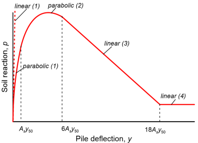
(6.139) $p = 0.5{p_f}{\left( {\dfrac{y}{{{y_{50}}}}} \right)^{0.5}} - 0.055{p_f}{\left( {\dfrac{{y - {A_s}{y_{50}}}}{{{A_s}{y_{50}}}}} \right)^{1.25}}{\rm{ \:for\: }}{A_s}{y_{50}} < y < 6{A_s}{y_{50}}$

Step 8:

Establish the next linear part of the p-y curve, named linear(3) in Figure 6.115, according to Eq. 6.140. It defines the softening part of the p-y curve from 6A_sy₅₀ up to pile deflection 18A_sy₅₀.

(6.140) $p = 0.5{p_f}{\left( {6{A_s}} \right)^{0.5}} - 0.411{p_f} - \dfrac{{0.0625}}{{{y_{50}}}}{p_f}\left( {y - 6{A_s}{y_{50}}} \right){\rm{ \:for\: 6}}{A_s}{y_{50}} < y < 18{A_s}{y_{50}}$

Step 9:

Establish the final linear part of the p-y curve, named linear(4) in Figure 6.115, using Eq. 6.141. This segment corresponds to the residual soil reaction, at large relative soil-pile displacements.

(6.141) $p = 0.5{p_f}{\left( {6{A_s}} \right)^{0.5}} - 0.411{p_f} - 0.75{p_f}{A_s}{\rm{\: for\: 18}}{A_s}{y_{50}} < y$

In many practical cases we can ignore the initial linear part of the curve, as intersection of linear(1) with the parabolic(1) part takes place at very small pile deflection (of the order of 1 mm). This would be the case for a 15-m long pile with diameter D = 0.5 m, driven in stiff clay with assumed constant undrained shear strength S_u= 100 kPa and submerged unit weight γ′= 6 kN/m³. The ultimate soil reaction per unit pile length can be estimated as:

(6.142) ${p_f} = \min \left\{ {\begin{array}{*{20}{c}}{100 + 6z + 283z}\\{550}\end{array}} \right\}{\rm{ }}\dfrac{{{\rm{kN}}}}{{\rm{m}}}$

whereas the factor A_s is calculated from the formulas depicted in Figure 6.114:

(6.143a) ${A_s} = 0.11\ln \left[ {\dfrac{z}{{0.5}} + 1} \right] > 0.2{\rm{ \:for\: }}z{\rm{ < 2 m}}$

(6.143b) ${A_s} = 0.6{\rm{ \: for \:}}z{\rm{ > 2 m}}$

where z is the depth from the ground surface. From Table 6.17 for undrained shear strength of clay S_u= 100 kPa we obtain a characteristic strain ε₅₀≈ 0.007 therefore y₅₀ = ε₅₀D = 0.003 m.

The expressions providing the distinct parts of the p-y curve are presented in Table 6.19.

**Table 6.19.** Expressions defining the *p-y* curves for a 15-m long pile embedded in stiff clay in the presence of free water, for z > 2m.
Lateral pile deflection, y (m)	Soil reaction, p (kN/m)
0 < y < 0.003A_s	$0.5{p_f}{\left( {\dfrac{y}{{0.003}}} \right)^{0.5}}$
0.003A_s< y < 0.018A_s	$0.5{p_f}{\left( {\dfrac{y}{{0.003}}} \right)^{0.5}} - 0.055{p_f}{\left( {\dfrac{{y - 0.003{A_s}}}{{0.003{A_s}}}} \right)^{1.25}}$
0.018A_s< y < 0.054A_s	$0.5{p_f}{\left( {6{A_s}} \right)^{0.5}} - 0.411{p_f} - 20.83{p_f}\left( {y - 0.018{A_s}} \right)$
y > 0.054A_s	$p = 0.5{p_f}{\left( {6{A_s}} \right)^{0.5}} - 0.411{p_f} - 0.75{p_f}{A_s}$
For z > 2 m it is p_f = 550 kN/m and A_s = 0.6

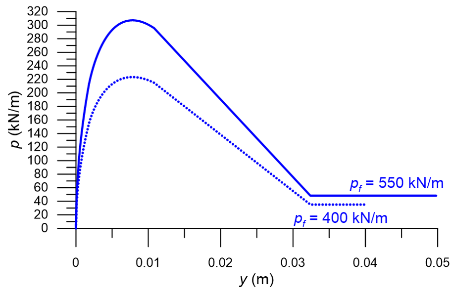
Notice from Eqs. 6.142 and 6.143 that in this particular case, both the factor A_s and the ultimate soil resistance do not change for the part of the pile embedded deeper than 2 m, thus the p-y response of the pile for z > 2 m will remain unaltered if the variation of the undrained soil strength with depth is not considered (Figure 6.116). Observe also in Figure 6.116 that the maximum soil reaction acting on the pile is not equal to p_f calculated from Eq. 6.136 (see also Eq. 6.139).

Variation of reaction p with pile deflection y, for different depth z <2 m and z > 2 m, measured from the soil surface. The ultimate reaction increases from pf = 400 kN/m to pf = 550 kN/m as z increases to z > 2m, but the deflection required to mobilise the ultimate and residual reaction is independent of z. — Figure 6.116. Indicative *p-y* curve for a 15-m pile embedded in stiff clay in the presence of free water, for z > 2m. The two curves correspond to different *p_f* values calculated from Eq. 6.136.

6.27.3 p-y curves for piles embedded in stiff clay, when no free water is present

Step 1:

Estimate the undrained shear strength of the clay S_u, and the characteristic strain ε₅₀ from laboratory undrained triaxial compression tests. If such tests are not available, ε₅₀ may be estimated from Table 6.17. Keep in mind that higher ε₅₀ values will result in more conservative predictions of pile response to lateral loads.

Step 2:

Compute the ultimate soil resistance per unit length of the pile as the minimum of two values:

(6.144) ${p_f} = \min \left\{ {\begin{array}{*{20}{c}}{\left( {3 + \dfrac{\gamma }{{{S_u}}}z + \dfrac{J}{D}z} \right){S_u}D}\\{9{S_u}D}\end{array}} \right\}$

where the factor J takes values J = 0.5 for soft clays and J = 0.25 for medium-to-firm clays.

Step 3:

Compute the deflection y₅₀ at one-half the ultimate soil reaction p = 0.5p_f:

(6.145) ${y_{50}} = 2.5\varepsilon {}_{50}D$

Step 4:

All the input parameters of the p-y curve have now been determined:

(6.146a) $p = 0.5{p_f}{\left( {\frac{y}{{{y_{50}}}}} \right)^{0.25}}{\rm{ for \: }}y < 16{y_{50}}$

(6.146b) $p = {p_f}{\rm{ \: for \:}}y \ge 16{y_{50}}$

The shape of the p-y curve is depicted in Figure 6.117.

For example, consider a 15-m long pile with diameter D = 0.5 m, driven in stiff clay with undrained shear strength S_u= 100 kPa and saturated unit weight γ_sat= 16 kN/m³. Assuming J = 0.5 and ε₅₀= 0.007, Eq. 6.144 yields:

(6.147) ${p_f} = \min \left\{ {\begin{array}{*{20}{c}}{\left( {3 + \dfrac{{16}}{{100}}z + \dfrac{{0.5}}{{0.5}}z} \right)100 \times 0.5 = 150 + 58z}\\{9 \times 100 \times 0.5 = 450}\end{array}} \right\}{\rm{ }}\dfrac{{{\rm{kN}}}}{{\rm{m}}}$

Further, substituting in Eq. 6.145:

(6.148) ${y_{50}} = 2.5\varepsilon {}_{50}D = 0.0087{\rm{\: m}}$

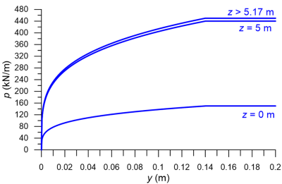
Notice from Eq. 6.147 that the ultimate soil resistance increases up to a depth z = 5.17 m, and remains constant for the part of the pile embedded in larger depths. For shallower depths, the variation of the ultimate soil resistance per unit length of the pile with depth z is given in Eq. 6.147. Indicatively, for z = 0:

(6.149) ${p_f} = \min \left\{ {\begin{array}{*{20}{c}}{150}\\{450}\end{array}} \right\}{\rm{ }}\dfrac{{{\rm{kN}}}}{{\rm{m}}}$

and the p-y curve at z = 0 is described by the function:

(6.150a) $p = 75{\left( {\dfrac{y}{{0.0087}}} \right)^{0.25}}{\rm{ }}\dfrac{{{\rm{kN}}}}{{\rm{m}}}{\rm{ \: for \:}}y < 0.14{\rm{ \:m}}$

(6.150b) $p = 150{\rm{ }}\dfrac{{{\rm{\:kN}}}}{{\rm{m}}}{\rm{ \: for \:}}y \ge 0.14{\rm{ \:m}}$

p-y curves along the length of the pile are illustrated in Figure 6.118:

Variation of reaction p with pile deflection y, for different depths z, measured from the soil surface z = 0 m, z = 5 m and z > 5.17 m. The ultimate reaction increases as z increases, but the deflection required to mobilise the ultimate reaction is independent of z. — Figure 6.118. Indicative *p-y* curves along a 15-m pile embedded in stiff clay when no free water is present.

6.27.4 p-y curves for a pile in sand above and below the water table

Step 1:

Determine the friction angle, φ′ of the sand, and its unit weight γ. Consider the submerged unit weight γ′ for sands below the water table (γ′ = γ – γ_w), and the bulk unit weight γ for sands above the water table.

Step 2:

Compute the ultimate soil reaction per unit length of the pile as the minimum of two values:

(6.151) ${p_f} = \min \left\{ {\begin{array}{*{20}{c}}{\left( {\gamma z} \right)\left[ {\dfrac{{{K_0}z\tan \varphi '\sin \beta }}{{\tan \left( {\beta - \varphi '} \right)\cos \alpha }} + \dfrac{{\tan \beta }}{{\tan \left( {\beta - \varphi '} \right)}}\left( {D + z\tan \beta \tan \alpha } \right) + {K_0}z\tan \beta \left( {\tan \varphi '\sin \beta - \tan \alpha } \right) - {K_a}D} \right]}\\{\left( {D\gamma z} \right)\left[ {{K_a}\left[ {\left( {{{\tan }^8}\beta } \right) - 1} \right] + {K_0}\tan \varphi '{{\tan }^4}\beta } \right]}\end{array}} \right\}$

Where α = φ′/2; β = 45⁰ + φ′/2; Κ₀ is the earth pressure coefficient at-rest recommended to be taken equal to K₀ = 0.6 for loose sand and K₀ = 0.4 for dense sand; K_A = active earth pressure coefficient K_A = tan²(45⁰ – φ′/2).

Step 3:

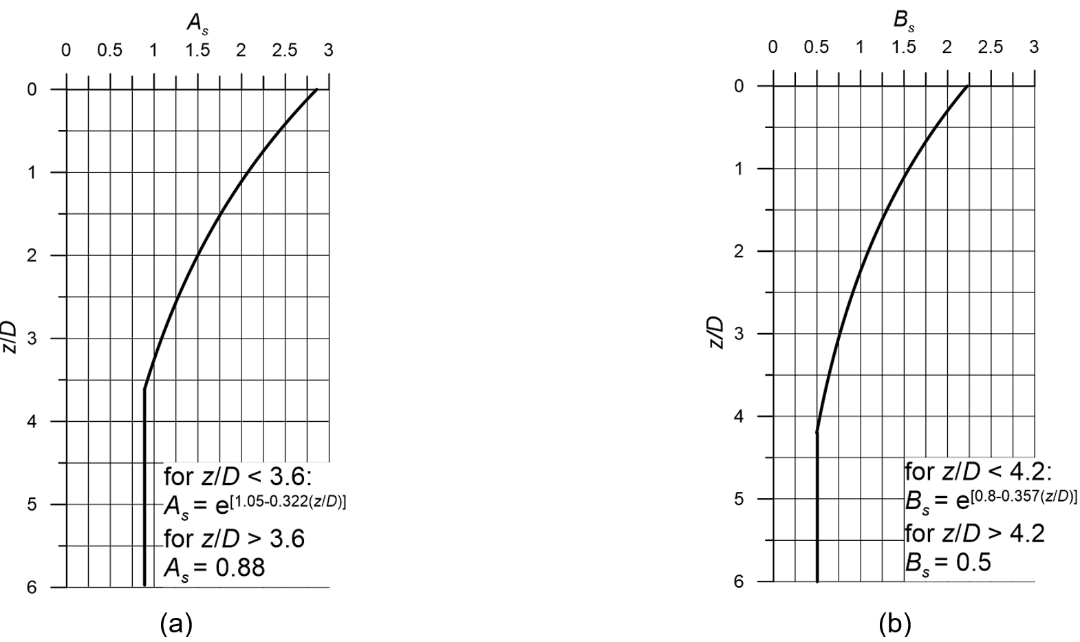
Use Figure 6.119a and the provided formulas to estimate the value of the factor A_s as function of depth measured from the soil surface z, and subsequently estimate the soil reaction developing when pile deflection reaches y₁ = 3D/80 as:

(6.152) ${p_1} = {A_s}{p_f}$

Figure (a) on the left presents the variation of the parameter As with dimensionless depth z/D. For z/D < 3.6 As is calculated as As = e^[1.05-0.322(z/D)] and for z/D > 3.6 As is constant As = 0.88. Figure (b) on the left presents the variation of the parameter Bs with dimensionless depth z/D. For z/D < 4.2 Bs is calculated as Bs = e^[0.8-0.357(z/D)] and for z/D > 4.2 Bs is constant Bs = 0.5. — Figure 6.119. Variation of factors (a) *A_s* and (b) *B_s* with normalized depth *z/D*; Piles in sand.

Step 4:

Use Figure 6.119b and the provided formulas to estimate the value of factor B_s as function of depth measured from the soil surface z, and subsequently estimate the soil reaction developing when pile deflection reaches y₂ = D/60 as:

(6.153) ${p_2} = {B_s}{p_f}$

Step 5:

Estimate the slope of the initial linear of the p-y curve, k_py from Table 6.20, depending on the relative density of the sand and groundwater table conditions.

**Table 6.20.** Slope of the initial linear part of the *p-y* curve for piles in sand above and below the water table (Reese and van Impe 2001).
Sand density	Sand below the water table	Sand above the water table
Sand density	k_py (static, kN/m³)	k_py (static, kN/m³)
Loose	5400	6800
Medium	16300	24400
Dense	34000	61000

Step 6:

Determine the factors m, n and C as:

(6.154) $m = \dfrac{{{p_1} - {p_2}}}{{{y_1} - {y_2}}}$

(6.155) $n = \dfrac{{{p_2}}}{{m{y_2}}}$

(6.156) $C = \dfrac{{{p_2}}}{{{{\left( {{y_2}} \right)}^{\tfrac{1}{n}}}}}$

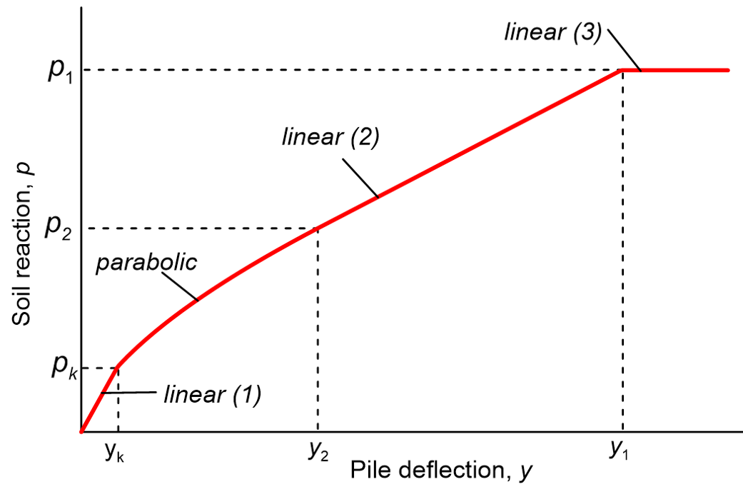
Step 7:

The p-y consists of three linear and one parabolic segment (Figure 6.120), described by the expressions listed in Table 6.21.

**Table 6.21.** Expressions describing the segments of the *p-y* curve for piles in sand above and below the water table (see Figure 6.120).
Segment (Figure 6.120)	Pile deflection range, y	Lateral resistance, p
linear (1)	$0 < y < {y_k} = {\left( {\dfrac{C}{{{k_{py}}z}}} \right)^{\left( {\tfrac{n}{{n - 1}}} \right)}}$	$p = {k_{py}}zy$
parabolic	${y_k} < y < {y_2} = \dfrac{D}{{60}}$	$p = C{y^{\tfrac{1}{n}}}$
linear (2)	${y_2} < y < {y_1} = \dfrac{{3D}}{{80}}$	$p = {p_2} + m\left( {y - {y_2}} \right)$
linear (3)	$y > {y_1}$	$p = {p_1}$

Graph presenting the different segments of a p-y curve. The segment linear (1) describes the p-y from zero deflection up to deflection yk. The segment parabolic describes the p-y curve from deflection yk up to deflection y2. The segment linear (2) describes the p-y curve from deflection y2 to deflection y1. The segment linear (3) describes the p-y curve for deflection larger than y1. — Figure 6.120. Segments of static *p-y* curve for a pile embedded in sand (after Reese *et al.*, 1974).

For example, consider a 15-m long pile with diameter D = 0.5 m, driven in medium-dense sand below the water table, with friction angle φ′ = 35º and submerged unit weight γ′ = 9.8 kN/m³. First, the soil resistance is estimated from Eq. 6.151, and accordingly A_s and B_sare calculated from the expressions provided in Figure 6.119. Assuming k_py= 24000 kN/m³ as an average value from Table 6.19 and K₀ = 0.4, we can obtain all the necessary parameters to determine the segments of the p-y curves from Table 6.21, for different elevations z along the pile. Indicatively, for depths z = 5, 10 and 15 m, the parameters of the curves are presented in Table 6.22, and the curves are plotted in Figure 6.121.

**Table 6.22.** Parameters of the *p-y* curves, for a 15-m pile embedded in sand below the water table.
z (m)	p_f,1(kN/m)	p_f,2(kN/m)	*A_s*	*B_s*	p₂(kN/m)	p₁(kN/m)	y_k(m)	y₂(m)	y₁(m)
5	811.5	1317.9	0.88	0.50	405.7	714.1	0.000835	0.00833	0.01875
10	3078.5	2635.8	0.88	0.50	1317.9	2319.5	0.002876	0.00833	0.01875
15	6801.1	3953.8	0.88	0.50	1976.9	3479.3	0.002876	0.00833	0.01875

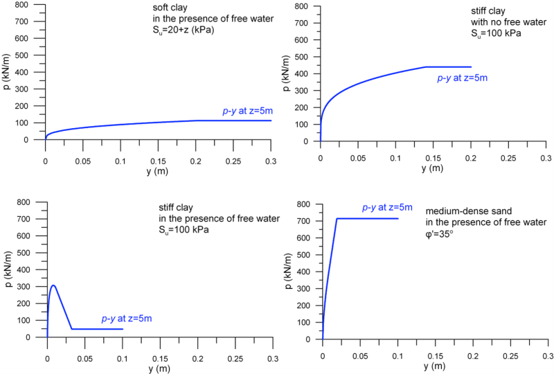
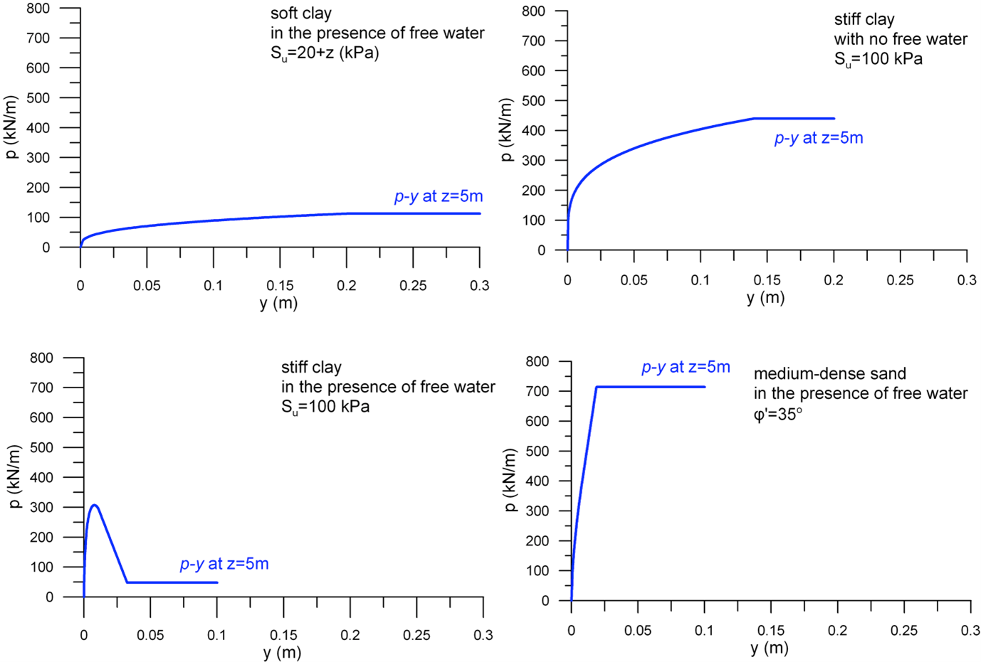
Variation of reaction p with pile deflection y, for different depths z, measured from the soil surface z = 5 m, z = 10 m and z = 15 m. The ultimate reaction increases as z increases, but the deflection required to mobilise the ultimate reaction is independent of z. — Figure 6.121. Indicative *p-y* curves along a 15-m pile embedded in dense sand below the water table.

A comparison of the indicative p-y curves presented in Figures 6.113, 6.116, 6.118 and 6.121 for clays and sands under variable groundwater table conditions is presented in Figure 6.122, for a typical depth below the ground surface z = 5 m. It is clear that the shape of the curves, and the ultimate reaction developing on the pile, strongly depend on the properties of the surrounding soil, and groundwater table conditions.

Four charts presenting p-y curves at depth z = 5 m for piles in different soils. The chart on the top left corresponds to pile in soft clay with Su = 20 + z (kPa) in the presence of free water. The chart on the top right corresponds to pile in stiff clay with Su = 100 kPa with no free water. The chart on the bottom left corresponds to pile in stiff clay with Su = 100 kPa in the presence of free water. The chart on the bottom right corresponds to pile in medium dense sand with φ' = 35 deg in the presence of free water. — Figure 6.122. Comparison of indicative *p-y* curves for different soil and groundwater conditions.

License

Icon for the Creative Commons Attribution 4.0 International License

Fundamentals of foundation engineering and their applications Copyright © 2025 by University of Newcastle & G. Kouretzis is licensed under a Creative Commons Attribution 4.0 International License, except where otherwise noted.

6.27.1 p-y curves for piles embedded in soft clay, in the presence of free water

6.27.2 p-y curves for piles embedded in stiff clay, in the presence of free water

6.27.3 p-y curves for piles embedded in stiff clay, when no free water is present

6.27.4 p-y curves for a pile in sand above and below the water table

License

Share This Book