6.12 Ultimate geotechnical strength of piles subjected to axial compressive load from CPT test results

George Kouretzis

6.12 Ultimate geotechnical strength of piles subjected to axial compressive load from CPT test results

Initially, the cone penetration test was developed exactly for the estimation of the collapse load of driven piles, and several methodologies have been proposed for the estimating pile capacity on the basis of measurements obtained from CPT tests performed at the proposed pile location. Most of these methods are based on determining the collapse load as the sum of the skin friction resistance along the pile shaft and the end-bearing resistance at the pile toe, similar to the α– and β-Method. As consequence the two key quantities that the Geotechnical Engineer is called to calculate is the (depth-dependent) skin friction stress along the pile, and the end-bearing resistance in terms of stress. It is not the aim of this section to provide a critical analysis of different methods, and endorse one over the other. The interested reader is referred to Schneider et al. (2008), Lehane et al. (2005a) and various other publications for a discussion on the advantages and prediction capabilities of the methods. Here the most widely used methods are presented, in chronological order, starting with Schmertmann’s method.

6.12.1 Schmertmann (1978) method for calculating the skin friction resistance

Despite being proposed almost 50 years ago, and the publication of several more refined methods since, Schmertmann’s (1978) method for estimating the skin friction resistance is still applied in practice, perhaps owing to its simplicity as well as its consideration of different pile materials. According to Schmertmann, the skin friction resistance ΔQ_sf (units: force/unit pile length) of a pile segment with length dL can be correlated to the sleeve penetration resistance from a CPT test f_s measured at the same depth as:

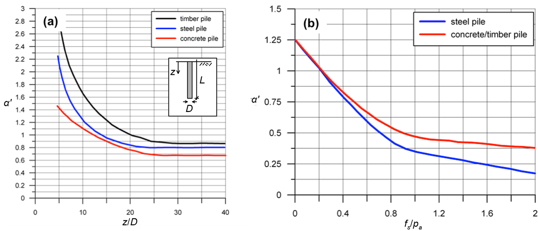
(6.23) $\Delta {Q_{sf}} = {f_{sf}}\left( {\pi D} \right)\Delta L = \left( {\alpha '{f_s}} \right)\left( {\pi D} \right)dL$

where α′ is a correction factor that depends on the material of the pile and the embedment ratio z/D for piles driven in coarse-grained soils, or the ratio of the CPT sleeve friction resistance over the atmospheric pressure f_s/p_a in fine-grained soils (Figure 6.23).

Instead of using the charts provided in Figure 6.23, one can use the following curve-fitting formulas for the estimation of the factor α′:

For concrete piles in coarse-grained soils (Figure 6.23a):

(6.24) $\alpha ' = 1.85 - 0.1\left( {\dfrac{z}{D}} \right) + 0.0025{\left( {\dfrac{z}{D}} \right)^2} - 0.259 \times {10^{ - 4}}{\left( {\dfrac{z}{D}} \right)^3}$

For steel piles in coarse-grained soils (Figure 6.23a):

(6.25) $\alpha ' = 3.88 - 0.482\left( {\dfrac{z}{D}} \right) + 0.0282{\left( {\dfrac{z}{D}} \right)^2} - 0.718 \times {10^{ - 3}}{\left( {\dfrac{z}{D}} \right)^3} + 0.668 \times {10^{ - 5}}{\left( {\dfrac{z}{D}} \right)^4}$

For concrete/timber piles in fine-grained soils (Figure 6.23b):

(6.26) $\alpha ' = 1.28 - 1.473\left( {\dfrac{{{f_s}}}{{{p_a}}}} \right) + 0.839{\left( {\dfrac{{{f_s}}}{{{p_a}}}} \right)^2} - 0.1634{\left( {\dfrac{{{f_s}}}{{{p_a}}}} \right)^3}$

For steel piles in fine-grained soils (Figure 6.23b):

(6.27) $\alpha ' = 1.29 - 1.606\left( {\dfrac{{{f_s}}}{{{p_a}}}} \right) + 0.846{\left( {\dfrac{{{f_s}}}{{{p_a}}}} \right)^2} - 0.159{\left( {\dfrac{{{f_s}}}{{{p_a}}}} \right)^3}$

Figure (a) on the left presents the variation of the parameter α' with the dimensionless depth z/D. Three curves are provided for timber pile, steel pile and concrete pile. An inset figure is used to define the pile's length as L, the pile's diameter as D, while z is measure from the ground surface. Figure (b) on the right presents the variation of the parameter α' with the dimensionless sleeve friction resistance fs/pa. Two curves are provided for steel pile and concrete/timber pile. — Figure 6.23. Correction factor α′ for the estimation of the skin friction resistance from CPT test measurements for (a) coarse-grained soils, and (b) fine-grained soils, under short-term undrained loading conditions.

Accordingly, the total pile skin friction resistance is calculated as the sum of the unit friction resistance for all pile segments dL:

(6.28) ${Q_{sf}} = \int\limits_0^L {\alpha '{f_s}\left( z \right)} \pi Ddz$

6.12.2 LCPC method (Bustamante and Gianeselli 1982)

Another widely used method is the one proposed by Bustamante and Gianeselli (1982), also know as the LCPC method. It is based on the statistical analysis of 197 pile load tests covering a wide range of soil conditions, and is applicable to both drilled shafts and driven piles.

The end-bearing resistance is estimated with the LCPC method as:

(6.29) ${Q_b} = {q_{c\left( {eq} \right)}}{k_c}{A_b}$

where q_c(eq)is an equivalent average cone resistance in the vicinity of the pile toe from the CPT test, calculated as shown below; k_cis a bearing capacity factor from Table 6.5 or, according to Briaud and Miran (1992), can be assumed equal to k_c= 0.6 for clays and silts and k_c= 0.375 for sands; A_b is the area of the pile base.

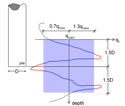
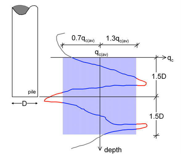
The equivalent average cone resistance q_c(eq)is estimated as illustrated in Figure 6.24 (Das 2007):

Consider the cone tip resistance q_c (or q_t if a piezocone test has been performed and cone resistance has been corrected for pore pressure effects) within a range of 1.5D below the pile toe to 1.5D above the pile toe.
Calculate the average value of the cone resistance q_c(av)within this zone.
Eliminate q_cvalues that are higher than 0.7q_c(av) and lower than 1.3q_c(av).
Calculate q_c(eq)by averaging the remaining q_c values.

**Table 6.5.** Bearing capacity factors *k_c* (after Bustamante and Gianeselli 1982, with modifications).
Soil type	Cone resistance q_c (MPa)	Factor k_c
Soil type	Cone resistance q_c (MPa)	Pile type I (drilled shafts)	Pile type II (driven piles)
Soft clay and mud	< 1	0.40	0.50
Moderately firm clay	1 to 5	0.35	0.45
Silt and loose sand	≤ 5	0.40	0.50
Firm to stiff clay and firm silt	> 5	0.45	0.55
Soft chalk	≤ 5	0.20	0.30
Medium dense sand/sand-gravel mixture	5 to 12	0.40	0.50
Weathered to fragmented chalk	> 5	0.20	0.40
Dense to very sand/sand-gravel mixture	> 12	0.30	0.40
Pile type I (Drilled shafts): Unreinforced drilled shafts; micropiles grouted under low pressure; cased drilled shafts; hollow auger drilled shafts, piers; barrettes
Pile type II (Driven piles): Cast in-place screwed piles; driven precast piles; prestressed tubular piles; driven cast piles; jacked steel piles; micropiles grouted under high pressure; driven grouted piles (low pressure grouting); driven steel piles; driven rammed piles; jacked concrete piles; high pressure grouted piles of large diameter > 250 mm

Schematic showing the variation with depth of cone resistance qc 1.5D above and 1.5D below the toe of a pile of diameter D. The average cone resistance along this stretch is defined as qc(av). A range extending between 0.7qc(av) and 1.3qc(av) is highlighted. Cone resistance qc values outside that range are marked with red and excluded from further calculations, while qc values within that range are used to calculated a revised average value. — Figure 6.24. Estimation of the equivalent average cone resistance *q_c(eq)* at the area of the pile toe.

In addition, the LCPC method can be used together with Eq. 6.23 and 6.28 to estimate the skin friction resistance (units: stress) from the distribution of the cone resistance q_c along the pile length as f_sf= q_c/α, with the coefficient α (instead of α′ in Eqs. 6.23 and 6.38) given in Table 6.6. Note that unlike the Schmertmann (1978) method described above, the LCPC method correlates the pile skin friction resistance to the cone tip resistance. Despite this being somewhat counterintuitive, it is considered an advantage by many due to difficulties in interpreting the CPT sleeve friction resistance f_s (Robertson and Kabal, 2022). As we will see in the next sections, this is followed by all modern methods.

**Table 6.6.** Skin friction resistance coefficient α (after Bustamante and Gianeselli 1982, with modifications).
Soil type	Cone resistance q_c(MPa)	Skin friction resistance coefficient α				Limiting value of skin friction resistance f_sf (kPa)
		Pile type				Pile type
		I		II		I		II		III
		A	B	A	B	A	B	A	B	A	B
Soft clay and mud	< 1	30	30	30	30	15	15	15	15	35	–
Moderately firm clay	1 to 5	40	80	40	80	35 to 80*	35 to 80*	35 to 80*	35	80	≥ 120
Silt and loose sand	≤ 5	60	150	60	120	35	35	35	35	80	–
Firm to stiff clay and firm silt	> 5	60	120	60	120	35 to 80*	35 to 80*	35 to 80*	35	80	≥ 200
Soft chalk	≤ 5	100	120	100	120	35	35	35	35	80	–
Medium dense sand/sand-gravel mixture	5 to 12	100	200	100	200	80 to 120*	35 to 80*	80 to 120*	80	120	≥ 200
Weathered to fragmented chalk	> 5	60	80	60	80	120 to 150*	80 to 120*	120 to 150*	120	150	≥ 200
Dense to very dense sand/sand-gravel mixture	> 12	150	300	150	200	120 to 150*	80 to 120*	120 to 150*	120	150	≥ 200
Pile type IA: Unreinforced drilled shafts; hollow auger drilled shafts; micropiles grouted under low pressure; cast in-place screwed piles; piers; barrettes
Pile type IB: Cased drilled shafts; driven cast piles
Pile type IIA: Driven precast piles; prestressed tubular piles; jacked concrete piles
Pile type IIB: Driven steel piles; jacked steel piles
Pile type IIIA: Driven grouted piles (low pressure grouting); driven rammed piles
Pile type IIIB: High pressure grouted piles of large diameter > 250 mm; micropiles grouted under high pressure
* Upper bound values apply to careful execution and minimum soil disturbance during construction

6.12.3 General about next generation CPT-based methods

More recently, the boom in construction of offshore facilities inspired among others the development of more rigorous (and perhaps less conservative) methods for the design of piles driven in silica sands and clays, including open-ended pipe piles for which soil plugging effects will be important. Some of the most popular of these methods, that rely heavily on CPT measurements, are compendiously presented in the following. The general form of the expression that provides the collapse load Q_f of a pile of constant diameter D is:

(6.30) ${Q_f} = {Q_{sf}} + {Q_b} - {W_p} = \pi D\int {{f_{sf}}\left( z \right)} dz + \left( {\dfrac{{\pi {D^2}}}{4}} \right){q_{bf}} - {W_p}$

where f_sf(z) is the depth-dependent skin friction resistance (units: stress), q_bf is the end-bearing resistance at the pile toe (units: stress) and W_p (units: force) is the weight of the pile, defined earlier. In this section we cover closed-end and open-ended (where soil plugging effects are important) piles subjected to axial compressive loads: estimation of the ultimate geotechnical strength or collapse load in tension is covered later in this Part.

6.12.4 FUGRO-05 method for piles in coarse-grained soils

The FUGRO-05 method (Kolk et al. 2005) has been developed by Fugro Engineers BV, a consulting firm with long experience in the design of offshore foundations. The skin friction resistance f_sf is calculated from the cone resistance q_c, similar to the LCPC method, as:

(6.31) ${f_{sf}} = 0.08{q_c}{\left( {\dfrac{{{{\sigma '}_{z0}}}}{{{p_a}}}} \right)^{0.05}}{\left( {\dfrac{h}{{{R^ * }}}} \right)^{ - 0.9}} {\rm{for} }{ {\dfrac{h}{{{R^ * }}}} {\ge}4}$

(6.32) ${f_{sf}} = 0.08{q_c}{\left( {\dfrac{{{{\sigma '}_{z0}}}}{{{p_a}}}} \right)^{0.05}}{\left( 4 \right)^{ - 0.9}}{\left( {\dfrac{h}{{4{R^ * }}}} \right)^{ - 0.9}}{\rm{for} }{ {\dfrac{h}{{{R^ * }}}} {<}4}$

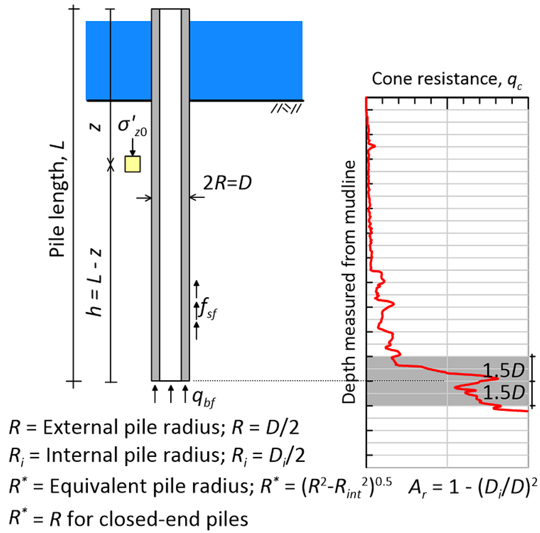
where σ′_z₀ is the vertical effective geostatic stress (again, the subscript ₀ refers to in situ conditions before installation of the pile) at depth z, p_a is the atmospheric pressure, while the remaining geometrical parameters are defined in Figure 6.25.

Schematic depicting an open-ended pipe pile of external radius R=D/2 and internal radius Ri=Di/2. The pile is partially embedded in soil, and its total length is L. A soil element is depicted at depth z, measured from the head of the pile, and the vertical effective stress at that pile element is denoted as σ'z0. The distance of that soil element from the pile toe is h = L-z. Friction stress fsf develop along the pile shaft, and end bearing stresses qbf develop at the pile toe. Two additional parameters are defined: the equivalent pile radius R*=(R^2-Rint^2)^(0.5) and A_r=1-(Di/D)^2. The variation of cone resistance qc along the depth, measured from the mudline, is plotted in a inset figure. A region extending 1.5D and 1.5D below the pile toe is highlighted. — Figure 6.25. Parameters introduced in the estimation of the compressive collapse load of offshore piles in sand with CPT-based methods.

The end-bearing resistance at the pile toe q_bf (units: stress) is calculated from the average cone resistance at the pile toe, q_c(av) which is determined according to Figure 6.24 as the average cone resistance over ± 1.5D from the pile toe (see also Figure 6.25):

(6.33) $\dfrac{{{q_{bf}}}}{{{p_a}}} = 8.5{\left( {\dfrac{{{q_{c\left( {av} \right)}}}}{{{p_a}}}} \right)^{0.5}}{A_r}$

where the area ratio A_r is calculated as (Figure 6.25):

(6.34) ${A_r} = 1 - {\left( {\dfrac{{{D_i}}}{D}} \right)^2}$

For solid piles it is of course A_r = 1. Note that the FUGRO method does not account for soil plug effects on the end-bearing resistance.

6.12.5 Imperial College ICP-05 method for piles in coarse-grained soils

The ICP-05 Method (Jardine et al. 2005) has been established from the analysis of field measurements obtained with the Imperial College Pile, a densely-instrumented kit developed at Imperial College, UK. For piles subjected to axial compressive load, the skin friction resistance (units: stress) f_sf is calculated as:

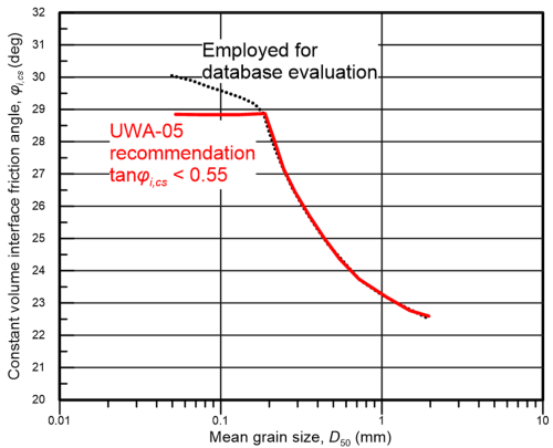
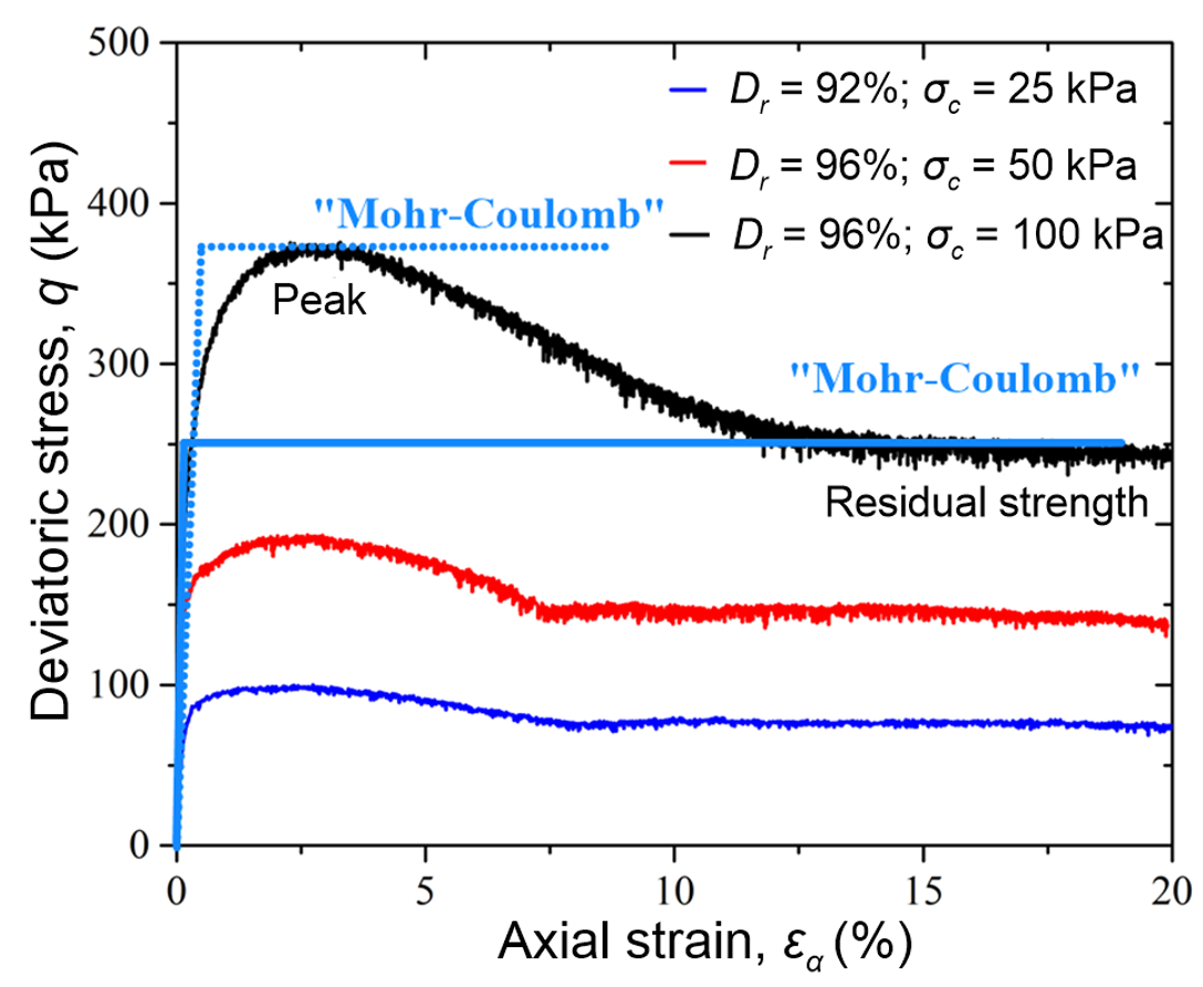
(6.35) ${f_{sf}} = {\sigma '_{hf}}\tan {\varphi _{i,cs}} = \left( {{{\sigma '}_{he}} + \Delta {{\sigma '}_{rd}}} \right)\tan {\varphi _{i,cs}}$

Whilst Eq. 6.35 features the same form as Eq. 6.10, the parameters introduced are different, and account for installation effects. First, instead of the peak interface friction angle φ_i, the skin friction resistance is correlated to the interface friction angle at constant volume (or at critical state) φ_i,cs, measured at large relative displacements when shearing at the soil-pile interface takes place under constant volume. This allows considering that slippage will take place along the soil-pile interface when the collapse load of the pile is reached, thus dilating sands will have reached their residual strength (see Figure 5.5). In lack of interface shear tests, Figure 6.26 can be used to obtain an estimate of φ_i,cs as function of the median grain size of sand D₅₀.

Graph presenting the variation of the constant volume interface friction angle φ'i,cs with mean grain size D50. According to UWA-05 recommendation tanφ'i,cs should be taken less than 0.55, regardless the mean grain size. — Figure 6.26. Variation of interface friction angle at constant volume φ_i,cs with median grain size *D₅₀* (after Lehane et al. 2005). UWA-05 method does not recommend using tanφ_i,cs values higher than 0.55.

In addition, Eq. 6.35 correlates skin friction resistance with the normal effective stress acting at the soil-pile interface when the collapse load is reached (or the pile fails) σ′_hf, and not the in situ geostatic horizontal effective stress σ′_h₀ as β-Method does. The normal effective stress at the soil-pile interface σ′_hf is calculated as the sum of the normal effective stress acting at the interface after pile installation and equalisation of pore pressures σ′_he, and the change in the normal stress acting at the interface that takes place during axial loading of the pile Δσ′_rd. This change in normal stress takes place as the pile expands radially when compressed, and is related to dilation at the soil-pile interface. σ′_hf is correlated to cone resistance q_c as:

(6.36) ${\sigma '_{hf}} = 0.029{q_c}{\left( {\dfrac{{{{\sigma '}_{z0}}}}{{{p_a}}}} \right)^{0.13}}{\left[ {\max \left( {\dfrac{h}{{{R^ * }}},8} \right)} \right]^{ - 0.38}}$

where all the symbols are defined in Figure 6.25. The change in normal stress during pile loading Δσ′_rd is calculated on the basis of cavity expansion theory as:

(6.37) $\Delta {\sigma '_{rd}} = 2G\left( {\dfrac{{\Delta r}}{R}} \right)$

where Δr is the interface dilation, which can be taken equal to Δr = 0.02 mm for slightly rusted steel piles, and G is the shear modulus of soil. Lehane et al. (2005) recommend using the low strain shear modulus G₀ together with Eq. 6.37, as soil deformations in the vicinity of the pile shaft are small. Monzon (2006) proposes to estimate G₀ from CPT measurements using a modified version of the expression of Baldi et al. (1989):

(6.38) ${G_0} = {q_c}1504.1{\left( {\dfrac{{{q_c}}}{{{{\sigma '}_{z0}}}}} \right)^{ - 0.7503}}$

For closed-end piles, the end-bearing resistance at the pile toe q_bf (units: stress) that develops when pile head displacement reaches about 10% of the pile’s diameter D is calculated again from the average cone resistance at the pile toe, q_c(av) as:

(6.39) ${q_{bf}} = {q_{c\left( {av} \right)}}\max \left[ {1 - 0.5\log \dfrac{D}{{{D_{CPT}}}},0.3} \right]$

where D_CPT = 35.7 mm is the standard cone diameter. Eq. 6.39 implies that the maximum pile diameter for which the formula works is of the order of D = 0.9 m, thus its use for larger piles is not recommended.

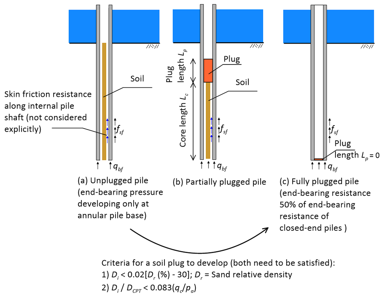
For open-ended pipe piles, the ICP-05 method employs different formulas for the calculation of q_bf, depending on whether the pile is completely plugged as consequence of arching (Figure 6.27c), or unplugged i.e., when soil coring takes place and there is relative movement between soil trapped inside the pile and the internal pile shaft (Figure 6.27a).

The figure on the left (a) shows a schematic of an unplugged pile, where end-bearing pressure is developing only at the annular pile base. The figure on the mid (b) shows a schematic of a partially plugged pile, with core length Lc (measured from the pile's toe) and plug length Lp. The figure on the right (c) shows a fully-plugged pile (Lp=0), for which the end-bearing resistance is taken to be 50% of the end-bearing resistance of closed-end piles. The criteria for a soil plug to develop are 1) Di<0.02[Dr (%) - 30] where Dr is the sand's relative density 2) Di/D_CPT < 0.083(qc/pa). Both criteria must be satisfied for the plug to develop. — Figure 6.27. Soil plugging in open-ended pile piles driven in sand.

An empirical criterion to determine whether there sufficient arching for the formation of a full plug will develop (Figure 6.27c) is show in Figure 6.27, and both conditions must be satisfied. If the criterion is satisfied, the end-bearing resistance will be 50% of the resistance calculated with Eq. 6.39, but no less than the end-bearing resistance that will develop at the annual pile base i.e.:

(6.40) ${q_{bf}} = {q_{c\left( {av} \right)}}\max \left[ {0.5 - 0.25\log \dfrac{D}{{{D_{CPT}}}},0.15,{A_r}} \right]$

where the pile’s area ratio A_r is defined in Eq. 6.34.

If the plugging criterion is not satisfied, then the pile should be considered as unplugged (Figure 6.27a) and the limiting end-bearing pressure is calculated as:

(6.41) ${q_{bf}} = {q_{c\left( {av} \right)}}{A_r}$

Note that the contribution of internal skin friction is not introduced explicitly into the calculation of the collapse load.

6.12.6 UWA-05 method for piles in sand

The UWA-05 method has been developed in the University of Western Australia by Lehane et al. (2005b), who reviewed the FUGRO-05, ICP-05 as well as the NGI-05 methods (not covered here for brevity), and subsequently established a unified set of recommendations which they tested against numerous pile load tests.

Calculation of the skin friction resistance f_sf (units: stress) that develops during axial compressive loading is based on the same concept as the ICP-05 method, and the same expression Eq. 6.35. However, calculation of the normal effective stress at the soil-pile interface at failure σ′_hf with the UWA-05 method is based on the following expression:

(6.42) ${\sigma '_{hf}} = 0.03{q_c}{\left( {{A_{r,eff}}} \right)^{0.3}}{\left[ {\max \left( {\dfrac{h}{D},2} \right)} \right]^{ - 0.5}}$

where A_r,eff is the effective area ratio, that depends on the so-called Incremental Filling Ratio IFR. IFR is a parameter that accounts for the displacement experienced by soil in the vicinity of the toe of open-ended piles during pile driving, when full or partial soil plugging (Figure 6.27) takes place during pile driving. As such A_r,eff is defined as:

(6.43) ${A_{r,eff}} = 1 - IFR{\left( {\dfrac{{{D_i}}}{D}} \right)^2}$

and the IFR is quantified as the increase in plug length with respect to the increase in pile’s driven length:

(6.44) $IFR = \dfrac{{\Delta {L_p}}}{{\Delta L}}$

where ΔL_p is the increment of soil plug length L_p corresponding to a small increment of the driven pile length ΔL (Figure 6.27). Fully plugged and fully coring modes correspond to IFR = 0 and IFR = 1 respectively, while intermediate values correspond to partially plugged piles. Eq. 6.43 requires as input the IRF corresponding to the final 20D of pile penetration which, in lack of site-specific data, can be approximated as:

(6.45) $IFR = \min {\left[ {1,\left( {\dfrac{{{D_i}}}{{1.5}}} \right)} \right]^{0.2}} \left( D_i {\rm \:in \: meters} \right)$

The change in normal stress during pile loading Δσ′_rd is calculated again with Eq. 6.37. Note that Lehane et al. (2005b) recommend the following expression, instead of Eq. 6.38, for calculating G₀ to be used together with Eq. 6.37:

(6.46) ${G_0} = {q_c}185{\left( {Q'} \right)^{ - 0.7}}$

Where:

(6.47) $Q' = \dfrac{{\left( {\dfrac{{{q_c}}}{{{p_a}}}} \right)}}{{{{\left( {\dfrac{{{{\sigma '}_{z0}}}}{{{p_a}}}} \right)}^{0.5}}}}$

is a dimensionless expression for cone resistance that has been introduced in Part 1.

The UWA-05 method does not differentiate the calculation of the end-bearing resistance at the pile toe q_bf (units: stress) for open and closed-end piles, as plugging effects are introduced by means of the filing ratio. The end-bearing resistance at the pile toe q_bf associated with pile head displacement about 10% of the pile’s diameter D is calculated as function of an alternative form of the average cone resistance at the pile toe, q_c(avD) as:

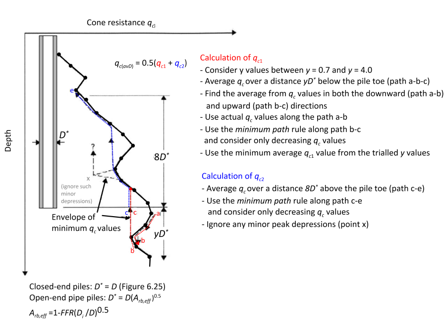
(6.48) ${q_{bf}} = {q_{c\left( {avD} \right)}}\left( {0.15 + 0.45{A_{rb,eff}}} \right)$

Instead of correlating q_bf to the average cone resistance at the pile toe q_c(av), Lehane et al. (2005b) recommend using the more complex “Dutch” averaging method described in Figure 6.28, and calculate q_c(avD) instead. The effective area ratio A_rb,eff is equal to A_rb,eff = 1 for closed-ended or fully-plugged piles, and can be calculated with the expression found in Figure 6.28. The Final Filling Ratio FFR in Figure 6.28 is the incremental filling ratio measured during the last stages of pile driving, and can be approximated again with Eq. 6.45.

Schematic showing the variation of cone resistance qc with depth along a pile with equivalent diameter D*. Cone resistance values across a depth ranging from 8D* above the pile toe and yD* below the pile are used for the calculation of the parameters qc2 and qc1 respectively. The parameter qc(avD) is calculated as qc(acD)=0.5(qc1+qc2). — Figure 6.28. Calculation of *q_c(avD)* with the Dutch averaging method (after Lehane *et al.* 2005).

6.12.7 ICP method for piles in fine-grained soils

The last CPT-based method for predicting the collapse compressive load of piles that is presented in this Chapter is the method developed by researchers at the Imperial College, UK (Jardine et al. 2005) on the basis on field tests with the Imperial College Pile ICP installed in clay-type soils. We refer to this as CPT-based method, despite the fact that the predicted skin friction resistance is independent of the cone resistance, but rather is function of the overconsolidation ratio, clay sensitivity, the geostatic vertical effective stress, and of course of the soil-pile interface friction angle.

The general formula Eq. 6.30 applies to this method too, and the expressions used to obtain the skin friction resistance f_sf and end-bearing resistance q_bf for piles driven in fine-grained soils are presented in the following. It must be stressed that, although the method provides a single expression for the short-term and long-term skin friction resistance, unlike the α-Method it is not based on total stress analysis but rather on effective stress principles. However, the effect of pore pressures that will develop during pile loading is accounted for, via the loading factor K_f/K_c.

The skin friction resistance is calculated with an expression similar to Eq. 6.35, as:

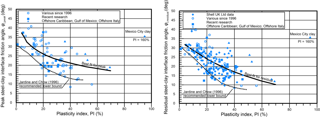
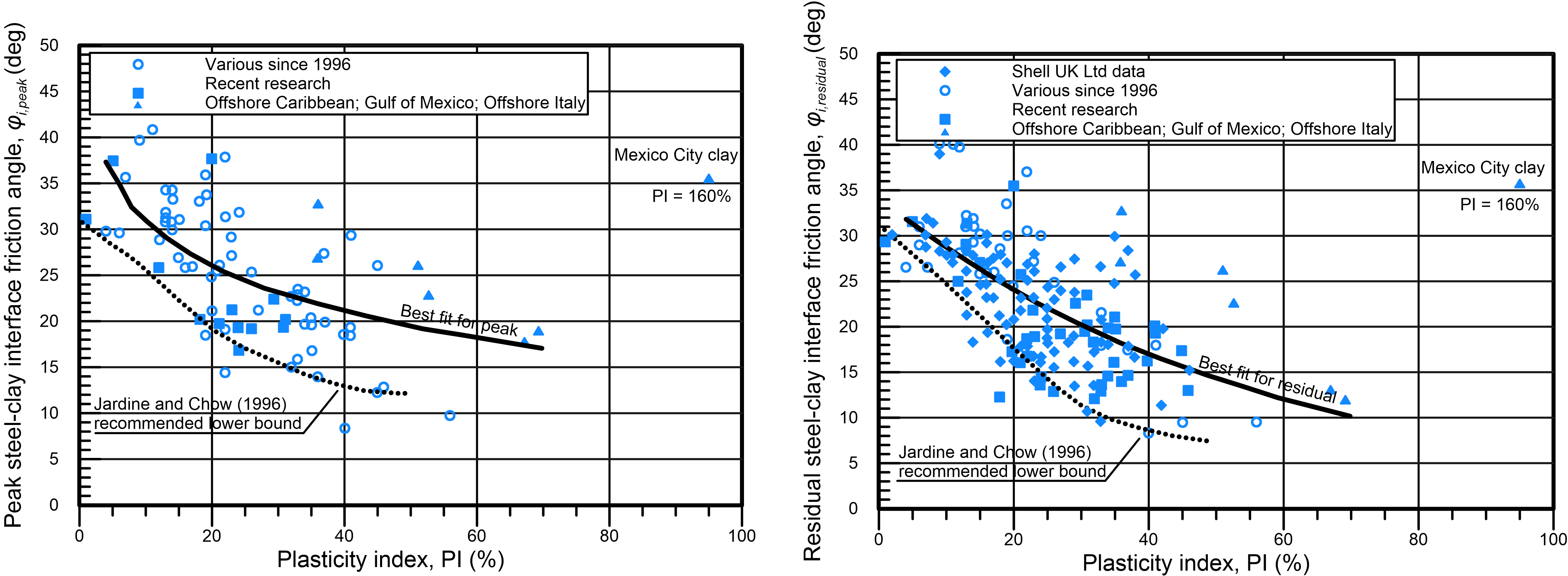
(6.49) ${f_{sf}} = {\sigma '_{hf}}\tan {\varphi _{i,f}} = \left( {\dfrac{{{K_f}}}{{{K_c}}}} \right){\sigma '_{he}}\tan {\varphi _{i,f}}$

where σ′_hf is the normal stress acting at the soil-pile interface at failure, while σ′_he is the normal stress acting at the soil-pile interface prior to pile loading and after equalisation of stresses induced during pile installation. φ_i,f in Eq. 6.49 is the interface friction angle at failure, and should be taken between the peak interface friction angle φ_i,peak and the residual φ_i,residual, which are both provided in Figure 6.29 as function of the plasticity index of clay PI. Of course a conservative approach is to consider φ_i,f = φ_i,residual.

For closed-end piles, the normal stress σ′_he acting at the soil-pile interface after equalisation is provided as function of the vertical in situ effective stress at the particular depth and a factor K_c as:

(6.50) ${\sigma '_{he}} = {K_c}{\sigma '_{z0}} = {\sigma '_{z0}}\left[ {2.2 + 0.016{\rm{OCR}} - 0.87\Delta {I_{vy}}} \right]{\rm{OC}}{{\rm{R}}^{0.42}}{\left[ {\max \left( {\dfrac{h}{R},8} \right)} \right]^{ - 0.20}}$

where OCR is the overconsolidation ratio, or (more rigorously, since stresses are not always vertical) the yield stress ratio YSR = σ′_vy/σ′_z0; ΔΙ_vy = log₁₀S_t is the logarithm of the clay’s sensitivity (Section 1.8.3); h/R is the normalised distance from the pile toe, defined in Figure 6.25. It is reminded here that for common clays that do not develop brittle shear bands upon shearing (S_u/σ′_z₀) = (S_u/σ′_z₀)_NCYSR^0.85 where S_u/σ′_z₀ is the undrained shear strength ratio in triaxial compression. Finally, the loading factor K_f/K_c in Eq. 6.49 accounts for the reduction in the normal stress acting at the soil-pile interface during loading of the pile, and it is taken equal to K_f/K_c = 0.8.

Figure (a) on the left presents values of the peak steel-clay interface friction angle, φi,peak, as function of the plasticity index. Different data points correspond to various data since 1996, recent research and offshore Caribbean, Gulf of Mexico and offshore Italy. Best fit line and lower bound line are provided. Figurer (b) on the right presents values of the residual steel-clay interface friction angle, φi,residual, as function of the plasticity index. Different data points correspond to Shell UK Ltd data, various data since 1996, recent research and offshore Caribbean, Gulf of Mexico and offshore Italy. Best fit line and lower bound line are provided. — Figure 6.29. (a) Peak and (b) residual soil-steel pile interface friction angle, determined via ring shear tests (after Jardine *et al.* 2005).

For open-ended piles, the normal stress σ′_he in Eq. 6.50 should be evaluated while considering the equivalent radius R* in Figure 6.25.

For closed-end piles, the end-bearing resistance at the pile toe q_bf (units: stress) that develops when pile head displacement reaches about 10% of the pile’s diameter D is calculated again from the average cone resistance at the pile toe, q_c(av) as:

(6.51) ${q_{bf}} = 0.8{q_{c\left( {av} \right)}}$ for short-term conditions (undrained loading)

(6.52) ${q_{bf}} = 1.3{q_{c\left( {av} \right)}}$ for long-term conditions (drained loading)

where the average cone resistance at the pile toe q_c(av) is determined according to Figure 6.24 as the average cone resistance over ± 1.5D from the pile toe (see also Figure 6.25).

For open-ended pipe piles, the ICP method employs different formulas for the calculation of q_bf, depending if the pile is completely plugged or unplugged. The criterion that must be satisfied for plugging to occur under static loading is:

(6.53) $\left[ {\dfrac{{{D_i}}}{{{D_{CPT}}}} + 0.45\left( {\dfrac{{{q_c}}}{{{p_a}}}} \right)} \right] < 36$

where D_CPT = 35.7 mm is the standard cone diameter. If the criterion is satisfied then q_bf is estimated to be half the resistance from Eqs. 6.51 and 6.52, or:

(6.54) ${q_{bf}} = 0.4{q_{c\left( {av} \right)}}$ for short-term conditions (undrained loading)

(6.55) ${q_{bf}} = 0.65{q_{c\left( {av} \right)}}$ for long-term conditions (drained loading)

If the criterion is not satisfied then coring will occur, and the limiting end-bearing pressure will develop only on the annular area of steel. In this case:

(6.56) ${q_{bf}} = {q_{c\left( {av} \right)}}{A_r}$ for short-term conditions (undrained loading)

(6.57) ${q_{bf}} = 1.6{q_{c\left( {av} \right)}}{A_r}$ for long-term conditions (drained loading)

where the area ratio A_r is defined in Eq. 6.34. As in the case of piles in sand, the contribution of internal skin friction is not introduced explicitly into the calculation of the collapse load.

License

Icon for the Creative Commons Attribution 4.0 International License

Fundamentals of foundation engineering and their applications Copyright © 2025 by University of Newcastle & G. Kouretzis is licensed under a Creative Commons Attribution 4.0 International License, except where otherwise noted.