6.10 Ultimate geotechnical strength of piles subjected to axial compressive load under drained conditions (β-Method)
The β–Method is used to analytically estimate the short-term and long-term collapse load Qf of piles installed in coarse-grained soils, and the long-term collapse load in fine-grained soils, under drained loading conditions, after excess pore pressures that will develop immediately after loading (careful, not installation) of the pile have dissipated. Calculation of the collapse load with the β–Method is based on effective stresses (Effective Stress Analysis-ESA). The concept introduced in the α-Method is followed here too i.e., skin friction and end-bearing resistance are considered separately, and the collapse load is calculated as the sum of the skin friction resistance and the end-bearing resistance of the pile (Eqs. 6.3-6.4).
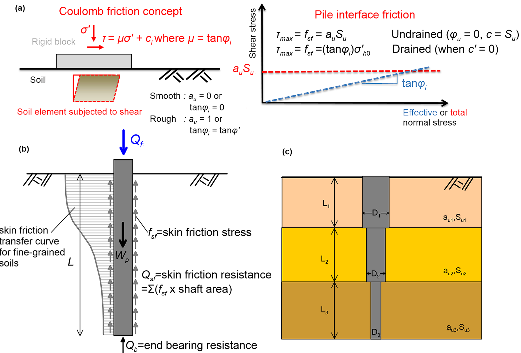
The skin friction is estimated in terms of effective stress while considering again that the Coulomb friction law describes the shear resistance that develops at the soil-pile interface (Figure 6.17a). Ignoring soil cohesion, the frictional stress along the shaft fsf is equal to the product of the lateral effective normal stress acting perpendicularly to the interface σ′h0, multiplied by a friction coefficient μ equal to tanφi, with φi being the interface friction angle as:
(6.10) 
Assuming geostatic conditions (the subscript 0 refers to in situ conditions before installation of the pile), the lateral effective stress is calculated as:
(6.11) 
so, the frictional stress can be re-written as:
(6.12) 
Replacing the product of the earth pressure coefficient at-rest K0 and of the friction coefficient tanφi with a single factor β yields:
(6.13) 
Notice that, as the vertical effective stress σ′z0 is not constant with depth, friction developing along the pile shaft is not uniform but rather increases with depth, while it depends also on groundwater table level.
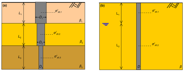
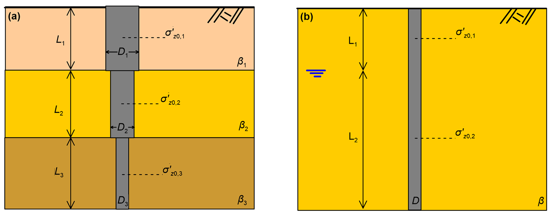
Considering the general case of multiple layers n (Figure 6.19a) and, for simplicity, the effective stress acting at the middle of each drained layer k, the skin friction resistance (units: force) along a pile of variable circular cross-section will be calculated as:
(6.14) 
In the case of a deep uniform drained layer with groundwater table present (Figure 6.19b), a better approximation of the skin friction resistance will be obtained if we divide the foundation soil into sublayers, and estimate the effective stress at the middle of each sublayer.
Calculation of the β factor requires estimating the earth pressure coefficient at-rest K0 and the friction coefficient tanφi. The former can be estimated from the formula proposed by Jaky (1944):
(6.15) 
where OCR is the overconsolidation ratio, φ′ is the friction angle of soil while the exponent m is often taken equal to m = 0.5. For normally consolidated clays (OCR = 1) and sands the above expression degenerates to:
(6.16) 
It is recommended to use Eq. 6.16 together with the critical state friction angle of soil, instead of the peak friction angle: K0=1-sinφcs (Jaky, 1944). The interface friction angle is correlated with the friction angle of the soil, as:
(6.17) 
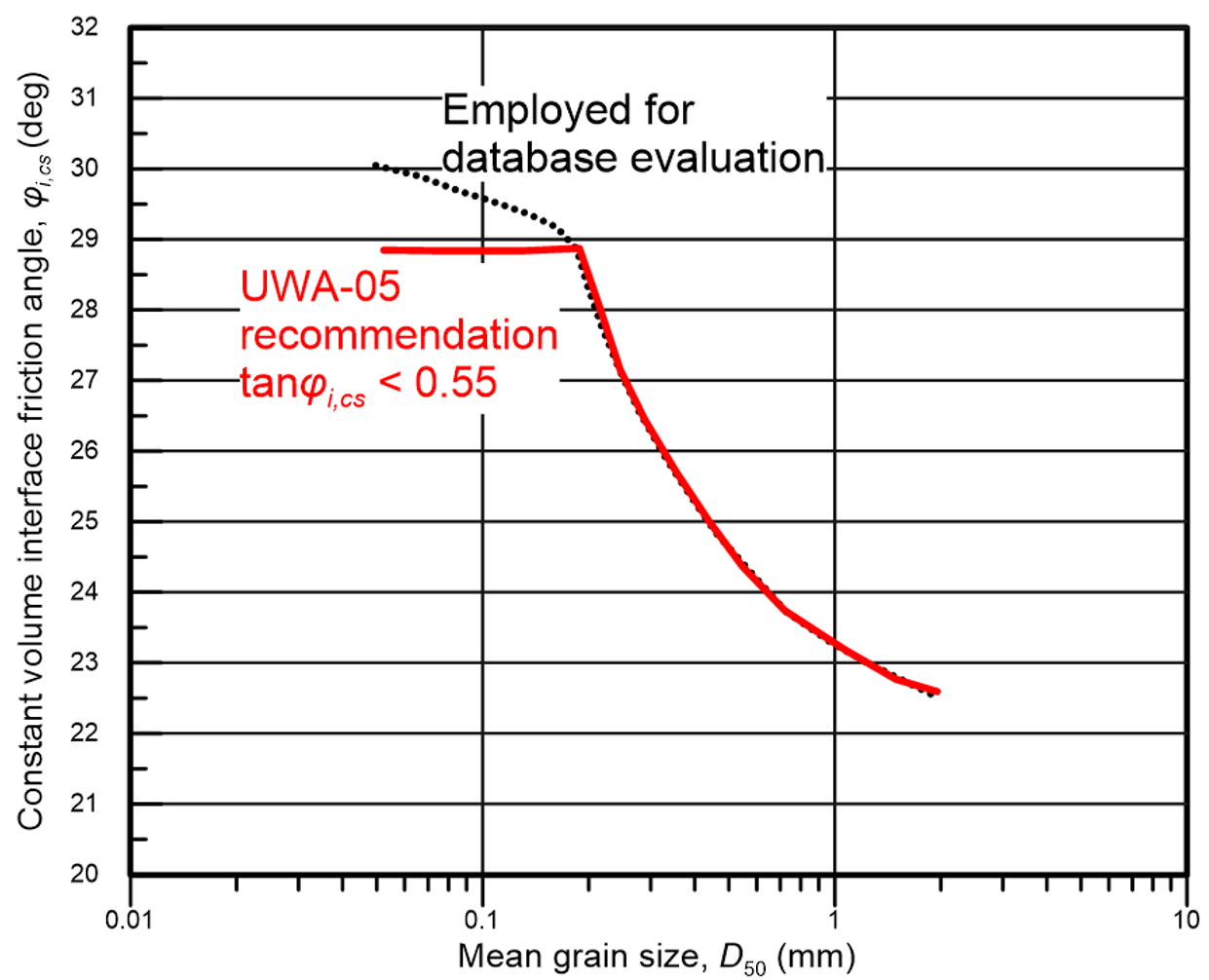
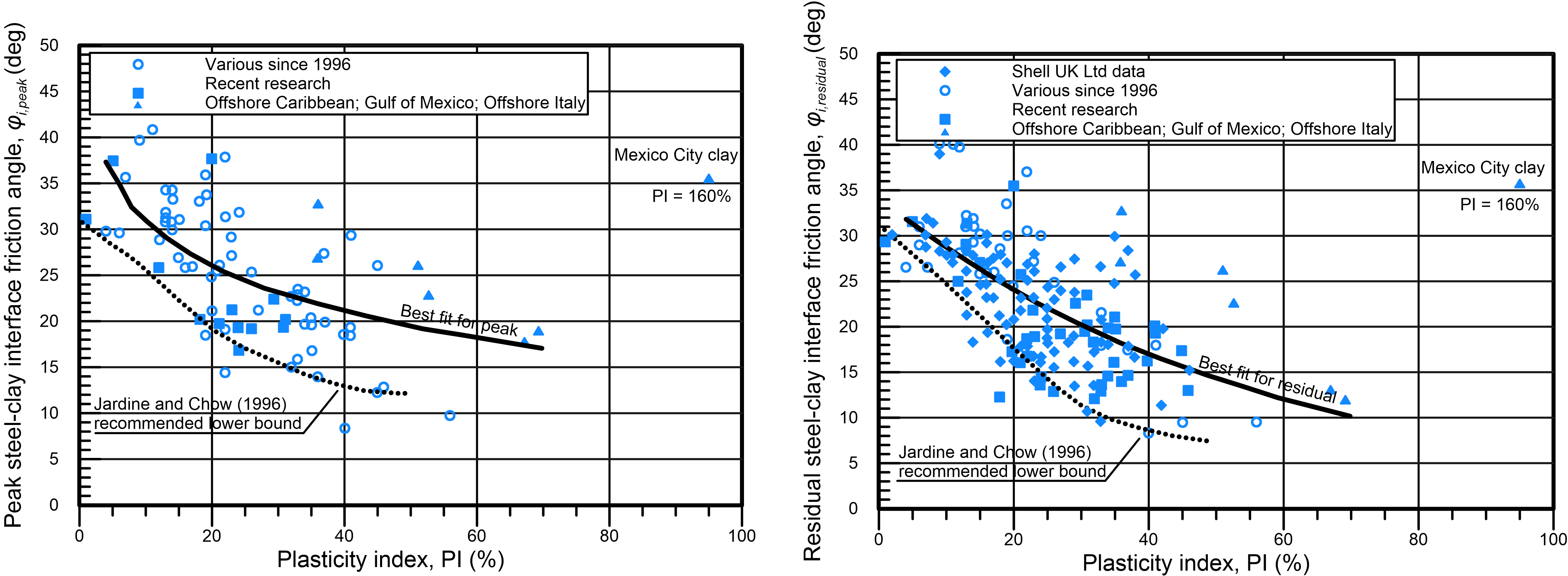
The upper bound value of φi/φ′ in Eq. 6.17 (see also Figure 6.17a) corresponds to a rather rough soil-pile interface, as the case of a concrete drilled shaft, while the lower bound value corresponds to a rather smooth soil-pile interface, as the case of a driven steel pile. Some further guidance on selecting appropriate φi values for piles driven in coarse-grained and fine-grained materials is provided in Chapter 6.12 (Figures 6.26 and 6.29).
While deriving the above expressions we have assumed that the normal stress acting at the soil-pile interface is equal to the geostatic stress σ′h0, in other words the pile is “wished in-place” and any soil disturbance effects due to driving are ignored. This is not going to be the case in practice, and the normal stress acting at the soil-pile interface will not be equal to the in situ lateral soil stress. Owing to disturbance induced from pile construction, Κ = σ′h/σ′z0 < Κ0 for drilled shafts due to stress relief during boring, and Κ > Κ0 for driven piles due to lateral stress increase during pile driving, where Κ is ratio of the normal stress acting at the soil-pile interface over the vertical geostatic effective stress. API RP2A (2000) suggests that, for driven piles, a value of σ′h/σ′z0 =0.8 to 1.0 describes better the lateral stresses developing at the interface. More rigorous methods for estimating σ′h are described in Chapter 6.12.
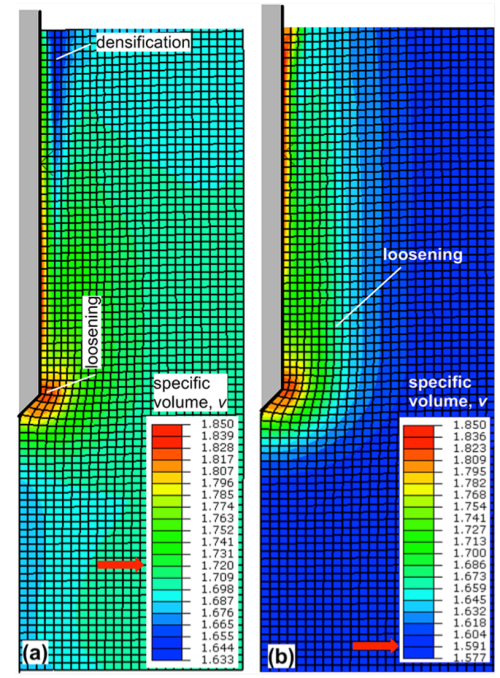
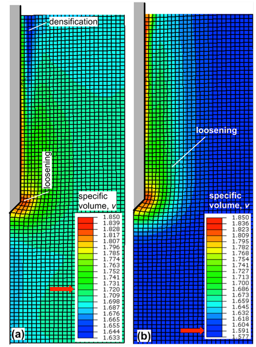
The friction angle of the soil around the pile will be also affected by pile driving, and generally will not be equal to the friction angle of the undisturbed soil, before pile construction. For example, friction angle of sand depends on its relative density. As pile driving will result in densification of a loose sand around the shaft, or perhaps to loosening of a dense sand (Figure 6.20) the friction angle may increase or decrease, respectively.
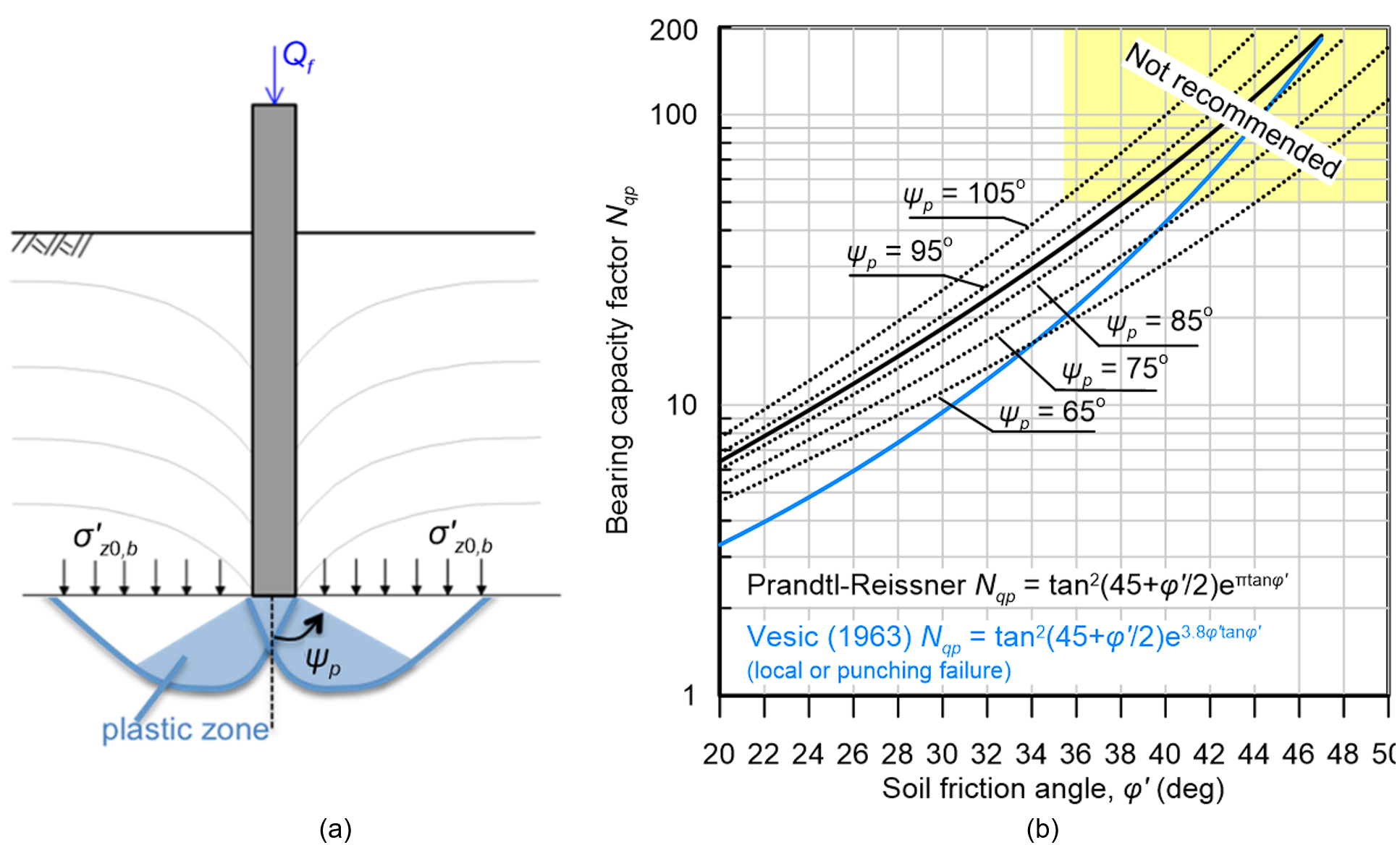
The end-bearing resistance Qb (units: force) is estimated similarly to the collapse load of shallow foundations under drained loading conditions (Figure 6.21a):
(6.18) 
where σ′z0,b is the vertical effective stress at the level of the pile toe, Ab is the area of the pile base and Nqp is the bearing capacity factor for drained conditions. The bearing capacity factor can be estimated either with the exact expression for shallow footings established originally by Reissner (1924):
(6.19) 
or, with the formula recommended in Janbu (1976), which takes into account the extent of the plastic zone developing below the pile toe, through the angle ψp:
(6.20) 
with ψp in rad. According to Bowles (1997), ψp ranges from 60º in soft clays to 105º in dense sands and overconsolidated clays. As depicted in Figure 6.21b, adopting the formula proposed by Reissner (1924) will result in an average value of the end-bearing resistance, compared to the range of values resulting from application of the Janbu (1976) formula.

The following Table 6.4 provides typical values provided by API RP2A (2000) of interface friction angle φi, skin friction stress fsf, drained bearing capacity factor Nqp and end-bearing resistance in terms of stress qbf = Qb/(σ′z0,bNqp). Values of fsf in Table 6.4 must be consider as indicative, as the skin friction resistance depends on depth (and groundwater), and are perhaps applicable to relatively long piles. It is worth noting that the maximum recommended Nqp factor is of the order of Nqp = 40 – 50. The author agrees with API RP2A (and with Vesic, who proposed a formula for Nqp that accounts for the possibility of local or shear failure, Figure 6.21b) in the sense that while Eq. 6.19 and 6.20 may yield Nqp values higher than Nqp = 50, adopting such values for pile design is not recommended. Remember that the friction angle of soils depends on the confining stress. Therefore, considering that high confining stresses are present at the pile toe (Chapter 6.6), it is prudent to consider a relatively conservative value of Nqp.
| Description | Density | φi (deg) | fsf (kPa) | Nqp | qbf = σ′z0,bNqp (MPa) |
|---|---|---|---|---|---|
| Sand; Silt; Silty sand/Sandy silt | Very loose to medium | 15 | 47.8 | 8 | 1.9 |
| Sand; Silt; Silty sand/Sandy silt | Loose to medium | 20 | 67.0 | 12 | 2.9 |
| Sand; Silty sand | Medium to dense | 25 | 81.3 | 20 | 4.8 |
| Sand; Silty sand | Dense to very dense | 30 | 95.7 | 40 | 9.6 |
| Sand; Gravels; Gravelly sand; Sandy gravels | Dense to very dense | 35 | 114.8 | 50 | 12.0 |
