5.4 Common bearing capacity equations and practical considerations
So far we have limited the discussion to idealised vertically-loaded strip and circular footings resting on the flat surface of semi-infinite, homogenous, isotropic, weightless soil. Under these assumptions we are able to derive exact solutions for the bearing capacity, but one may argue that these conditions, particularly weightless soil, are never met in practice. This is true, but we can use the above solutions together with correction factors for the effect of soil self weight, footing shape (for rectangular or square footings), load inclination and eccentricity, embedment conditions and groundwater table levels and estimate the design capacity required by AS 5100.3.
The net (i.e., not accounting for the contribution of overburden soil) bearing capacity (units: stress) equation for total stress analysis (TSA) under undrained conditions is:
(5.20) 
The net bearing capacity equation (units: stress) for effective stress analysis (ESA) under drained conditions is:
(5.21) ![q = \left[ {\gamma {D_f}\left( {{N_q} - 1} \right)} \right]{s_q}{d_q}{i_q}{b_q}{g_q} + \left[ {0.5\gamma B'{N_\gamma }} \right]{s_\gamma }{d_\gamma }{i_\gamma }{b_\gamma }{g_\gamma }](https://oercollective.caul.edu.au/app/uploads/quicklatex/quicklatex.com-71e3dacb04faba5ddf74d0e0c3619fd4_l3.png "Rendered by QuickLaTeX.com")
All symbols in the above equations will be introduced in the following. The above Eq. 5.20 conservatively disregards the beneficial contribution of soil cohesion c′, which is unlikely to be important in coarse-grained materials and non-cemented clays. As it is discussed in Example 5.1, when the footing is embedded into the soil at a depth Df, the bearing capacity is found by adding the weight of the excavated soil to the net bearing capacity q determined by Eqs. 5.20 and 5.21 as:
(5.22) 
Of course when a footing is not embedded in soil it is qf = q. Note that when using AS5100.3 provisions for the design of the foundation, the geotechnical strength reduction factor φg must be applied only on the net bearing capacity q to obtain the design capacity as:
(5.23) 
or φgRug ≠ (φgqf) x (area of footing). This is due to the fact that the uncertainties related to the weight of the excavated soil are considerably less than the uncertainties related to the shear failure developing in the soil below the footing.
Net bearing capacity Eqs. 5.20 and 5.21 include correction factors for the shape of rectangular or square footings (s), the effect of the embedment depth (d), the inclination of the load (i), the inclination of the base of the footing (b), the inclination of the foundation level (g) etc. Herein we focus on two of the most common cases of practical interest: i) a vertical load acting on a horizontal base footing resting on horizontal ground (Figure 5.22), and ii) an inclined load acting on a horizontal base footing resting on horizontal ground (Figure 5.30). In those cases, Eqs. 5.20 and 5.21 are simplified as follows:

Case (1) Vertical load on horizontal base footing resting on horizontal ground:
(5.24) 
(5.25) ![{\rm{Effective \:Stress \:Analysis \:ESA: \:}}q = \left[ {\gamma {D_f}\left( {{N_q} - 1} \right)} \right]{s_q}{d_q} + \left[ {0.5\gamma B'{N_\gamma }} \right]{s_\gamma }{d_\gamma }{\rm{ }}](https://oercollective.caul.edu.au/app/uploads/quicklatex/quicklatex.com-c14e2fdb3e9b4765947b3d2e6124126d_l3.png "Rendered by QuickLaTeX.com")
where: Nq, Nγ are the bearing capacity factors, accounting for the shear strength of soil; sc, sq, sγ are the shape factors; dc, dq, dγ are the embedment factors; γ is the unit weight of the foundation soil; B′ is the effective footing width, defined in the following.
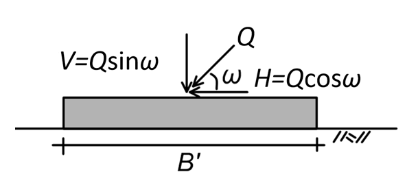
Case (2) Inclined load on horizontal base footing resting on horizontal ground:
(5.26) 
(5.27) ![{\rm{Effective \:Stress \:Analysis \:ESA: \:}}q = \left[ {\gamma {D_f}\left( {{N_q} - 1} \right)} \right]{i_q} + \left[ {0.5\gamma B'{N_\gamma }} \right]{i_\gamma }](https://oercollective.caul.edu.au/app/uploads/quicklatex/quicklatex.com-d32a1b166c28867e6e918103c3e8b516_l3.png "Rendered by QuickLaTeX.com")
where: Nq, Nγ are the bearing capacity factors, as above; ic, iq, iγ are the load inclination factors.
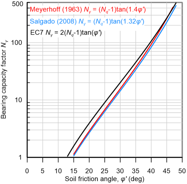
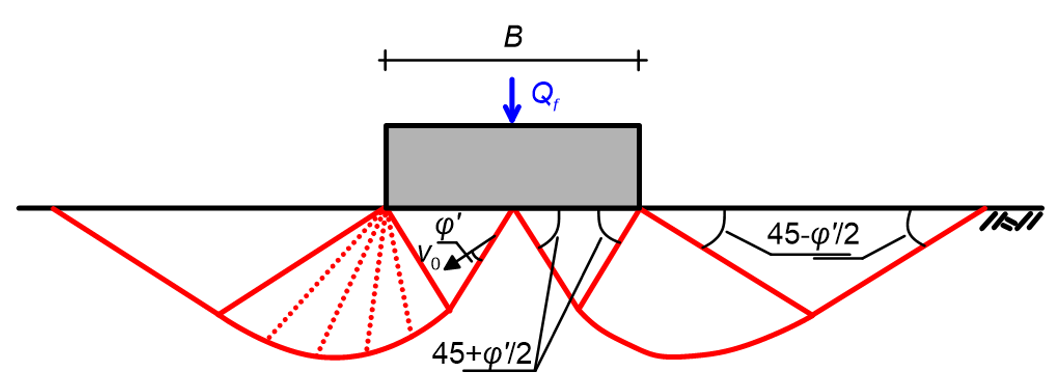
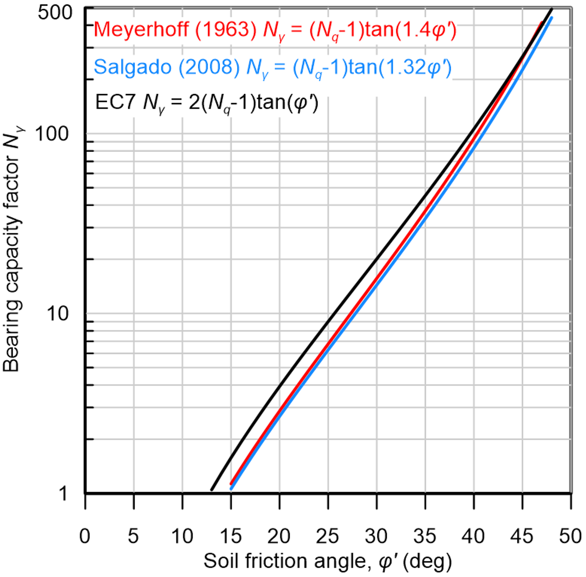
The bearing capacity factors are employed in effective stress analyses, considering drained soil response, and depend on the friction angle of the soil. Factor Nq is provided from the exact solution for weightless c′–φ′ soil (Eq. 5.18), considering the general failure mechanism depicted in Figures 5.23a and 5.28. On the other hand, there is no exact solution for soil with unit weight γ > 0 and various approximate expressions have been proposed for determining the corresponding bearing capacity factor Nγ, some of which are plotted in Figure 5.31. The expression that will be used mostly here is the one proposed by Meyerhoff (1963) for a rough footing:
(5.28) 
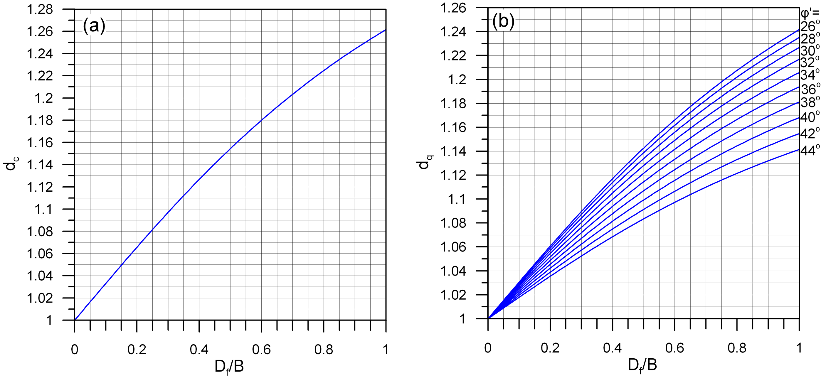
The expressions providing the shape and embedment factors both for total stress analysis (Eq. 5.24) and effective stress analysis (Eq. 5.25) are presented in Table 5.5, while the variation of the embedment factors dc and dq with the normalised embedment depth Df/B is also depicted in Figure 5.32.
| Total Stress Analysis (Eq. 5.24) | |
|---|---|
| sc |  |
| dc |
|
| Effective Stress Analysis (Eq. 5.25) | |
| sq |  |
| dq |  |
| sy |  |
| dy | 1 |


The load inclination factors, to be used together with Eqs. 5.26 and 5.27 are provided in Table 5.6. These expressions are valid for a load inclined at the plane defined by B′, as shown in Figure 5.30. Note that load inclinations factors are not to be used together with shape and embedment factors, so if e.g., an inclined load acts on an embedded footing, Eqs. 5.26 and 5.27 should be used.
| Total Stress Analysis (Eq. 5.26) | |
|---|---|
| ic |  |
| Effective Stress Analysis (Eq. 5.27) | |
| iq |  |
| iy | 1 |

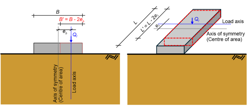
In the above formulas for the net bearing capacity and the correction factors, the effective width B′ and the effective length L′ of the footing are used, instead of their actual dimensions. The footing dimensions are adjusted to their effective values when the location of the resultant load (load axis) does not coincide with the centroid (centre of area) of the footing, so as to align the load centre with the area centre (Figure 5.33). The distance from the centre of the area to the point of application of the vertical component of the resultant load is called eccentricity, e. Given the eccentricity of the load, the effective width of a strip footing is:
(5.29) 
In the case of a rectangular footing, the same applies for the effective length:
(5.30) 
(a) (b)
Apart from the above, bearing capacity equations must be adjusted to account for groundwater effects, when performing an effective stress analysis under drained conditions. For that, we distinguish three cases, with respect to the elevation of the groundwater table relatively to the foundation level (Figure 5.34).
When the groundwater table is found below a depth B from the foundation level Df (Case 1, Figure 5.34) no reduction of the bearing capacity is necessary, as we can assume that the failure surface will be contained in the soil above the groundwater table. When the groundwater is found at a level above B+Df from the ground surface, its effect on the bearing capacity of the footing is introduced in Eq. 5.25 as:
Case 2, Figure 5.34:
(5.31) ![q = \left[ {\gamma {D_f}\left( {{N_q} - 1} \right)} \right]{s_q}{d_q} + \left[ {0.5\left\{ {\gamma z + \left( {\gamma - {\gamma _w}} \right)\left( {B' - z} \right)} \right\}{N_\gamma }} \right]{s_\gamma }{d_\gamma }](https://oercollective.caul.edu.au/app/uploads/quicklatex/quicklatex.com-e33cb225d55c84417ff214dbbfcf90c9_l3.png "Rendered by QuickLaTeX.com")
where z is measured from the foundation level of the footing.
Case 3, Figure 5.34:
(5.32) ![q = \left[ {\left\{ {\gamma z + \left( {\gamma - {\gamma _w}} \right)\left( {{D_f} - z} \right)} \right\}\left( {{N_q} - 1} \right)} \right]{s_q}{d_q} + \left[ {0.5\left( {\gamma - {\gamma _w}} \right)B'{N_\gamma }} \right]{s_\gamma }{d_\gamma }](https://oercollective.caul.edu.au/app/uploads/quicklatex/quicklatex.com-9e15579778f218065837570577e33523_l3.png "Rendered by QuickLaTeX.com")
where in this case z is measured from the soil surface.
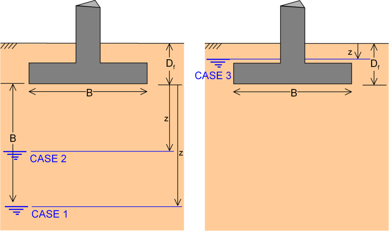
The above Eqs. 5.31 and 5.32 were simplified on the basis of the assumption that soil above the groundwater table is saturated, so its unit weight is equal to the saturated unit weight γ = γsat. Moreover, γw is the unit weight of water γw ≈ 10 kN/m3.
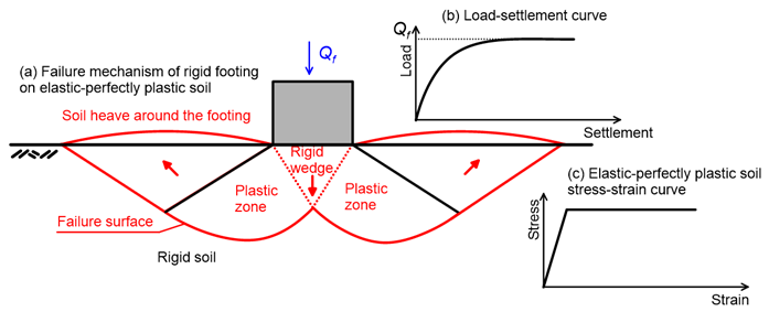
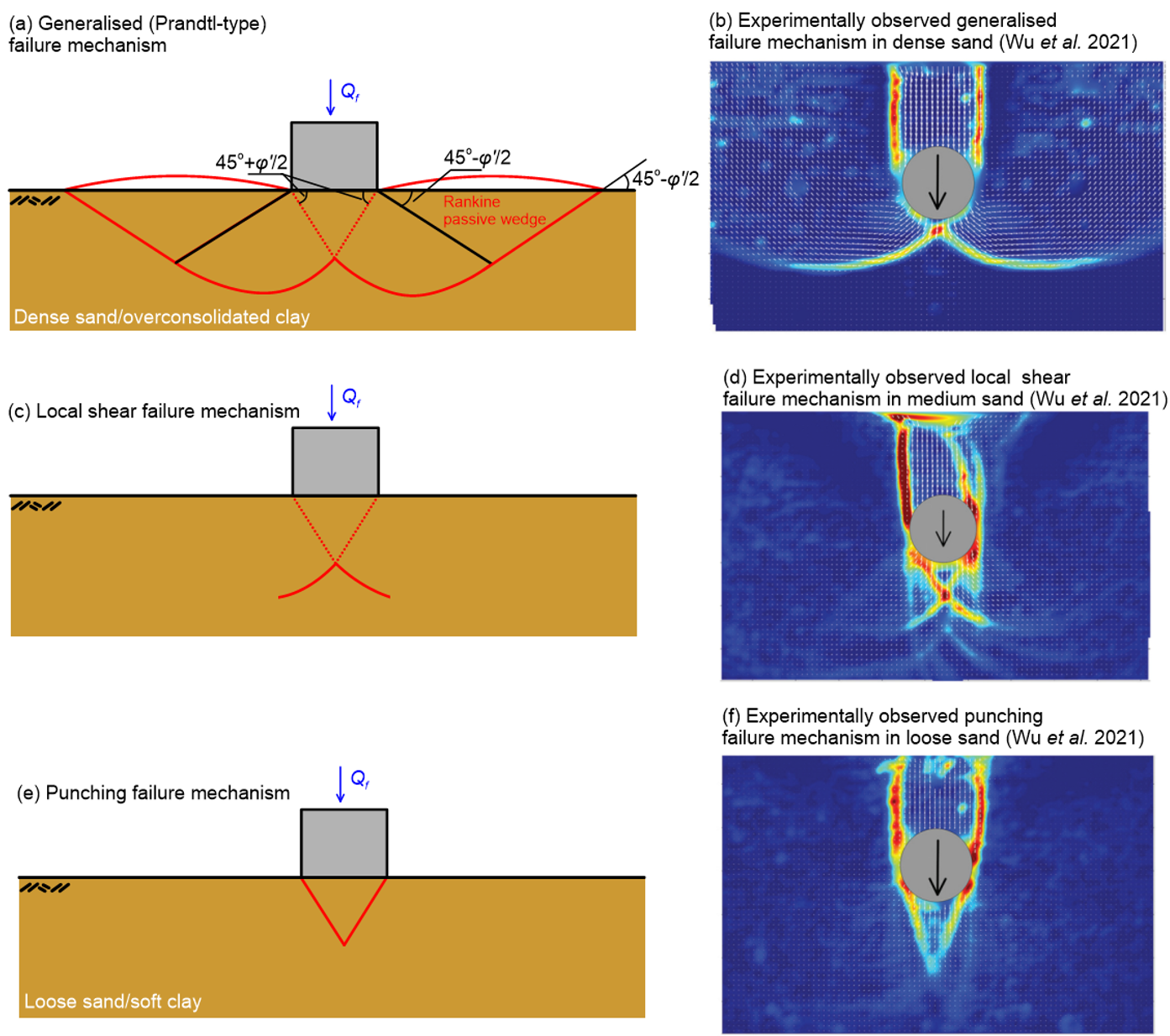
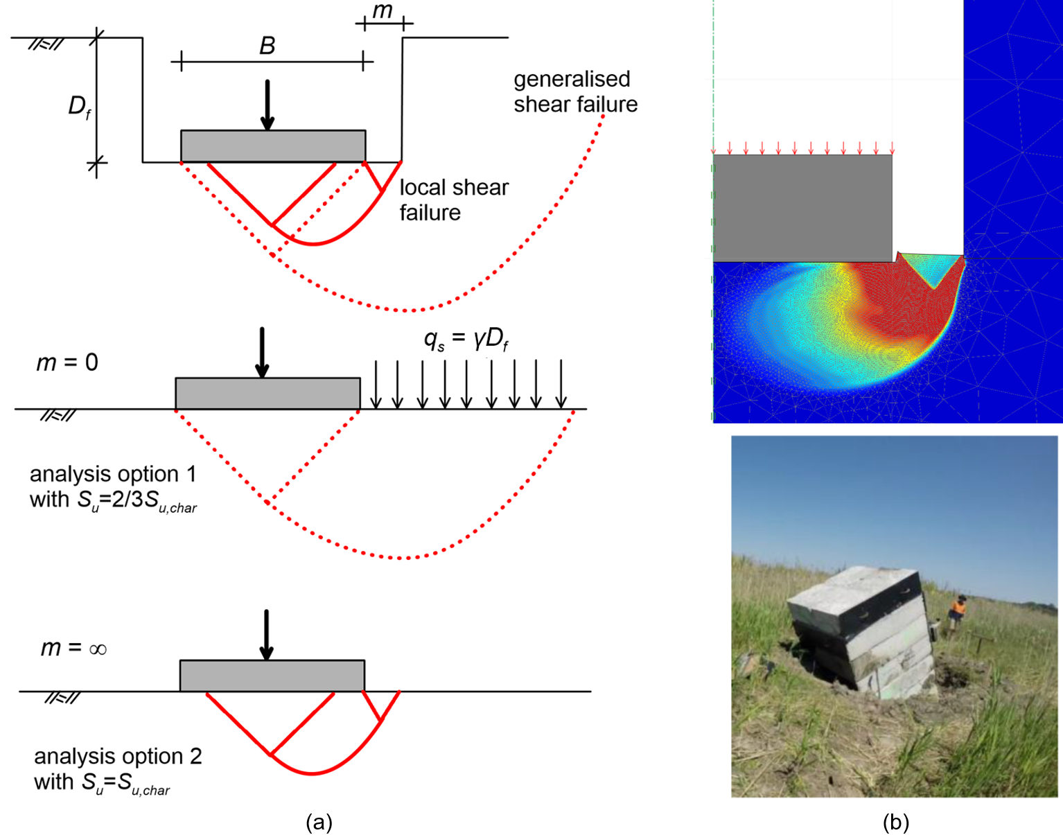
Finally, one of the main assumptions that we make when using all the expressions presented above is that a general shear failure mechanism (Hill- or Prandtl- type) will develop when the footing is loaded to failure. However, as discussed earlier and depicted in Figure 5.23, other failure mechanisms may develop in e.g., medium-dense sands (local shear mechanism, Figure 5.23b) or very soft clays/loose sands (punching mechanism, Figure 5.23c).
Consider for example the problem of estimating the bearing capacity of a footing embedded in a trench, when the footing is separated by the trench walls by a gap with width m. This scenario is not compatible with the assumptions of the analytical solutions presented above, and we cannot know whether a generalised or a local shear failure will develop if the footing is loaded up to its collapse load. Certainly, if we neglect the existence of the gap and assume that a generalised failure surface will develop with the soil overburden contributing beneficially to the bearing capacity, we are not on the safe side.
To address this, for footings on loose-to-medium sands with relative density Dr < 65% and soft clays with undrained shear strength Su < 50 kPa, where local shear failure is more likely to develop, it is proposed to use the bearing capacity expressions provided in this section while conservatively reducing the values of φ′ and Su to 2/3 of the characteristic value (Figure 5.35a, option 1):
(5.33) 
(5.34) 
Alternatively, we can completely ignore the existence of the overburden, assuming therefore a localised failure mode (Figure 5.35a, option 2). The above are in agreement with field tests performed by Gaone et al. (2017) on footings on soft clay, and numerical simulation results obtained by the author (Figure 5.35b). For the particular tests, both options 1 and 2 provided reasonably accurate estimates of the measured collapse load.

