5.2 Some fundamentals: Load and Resistance Factor Design (LRFD) & Shear strength of soils

George Kouretzis

5.2 Some fundamentals: Load and Resistance Factor Design (LRFD) & Shear strength of soils

5.2.1 General concepts

Geostructures are designed at the Ultimate Limit State to be able to safely carry a collapse load, without failure in the form of bearing capacity failure of shallow or deep foundations, rotational failure of slopes etc. Two design approaches are encountered in practice:

In the (perhaps now obsolete) conventional, allowable stress design (or Limit State Design) method, the collapse load is determined via analytical methods or numerical analyses, using appropriately factored material parameters. Accordingly, the collapse load or the load that a structure can safely carry at the Ultimate Limit State is divided by a Factor of Safety (F.S.) to obtain the allowable design load:

(5.1) ${\rm{Allowable \:design \:load = }}\dfrac{{{\rm{Collapse \:load}}}}{{{\rm{F}}{\rm{.S}}{\rm{.}}}}$

Values of the factor of safety depend on the nature of the problem, and are based on experience from previous projects. Thus, they are purely empirical.

Load and Resistance Factor Design, which forms the basis of design of foundations and soil-supporting systems with AS5100.3, but also with most modern geotechnical design codes from the United States and Europe, is based on reliability concepts and allows considering uncertainties in loads, soil resistance, method of analysis, and construction. The loads and action effects are multiplied by load factors (usually) greater than one, in different combinations, to determine the design action load S*. The ultimate geotechnical strength R_ug(in the context of this Part it is the compressive loading that the geostructure can safely carry at the Ultimate Limit State) determined analytically or numerically, is multiplied by a geotechnical strength reduction factor φ_g(usually) less than one, to provide the design capacity. Design of any geostructure at the Ultimate Limit State must satisfy the following inequality:

(5.2) ${\varphi _g}{R_{ug}} \ge {S^ * }$

or, according to AS5100.3 for shallow footings:

“Footings subjected to vertical or inclined loads or overturning moments shall be proportioned such as the design bearing capacity is greater than or equal to the design action effect S*”

Note here that the load and strength reduction factors apply only to strength calculations. Settlement calculations are performed while considering serviceability load combinations, and no geotechnical strength reduction factors are applied on the calculated settlement value.

5.2.2 Establishment of the design action load

Apart from the usual loads and surcharges, which are defined in AS1170.0 and AS1170.1 and discussed elsewhere, secondary loads must be considered for the design of geotechnical structures. These include loads resulting from vertical and lateral soil movement (e.g., negative skin friction due to consolidation, heave due to moisture changes in expansive soils), earth pressure loads, hydrostatic pressure loads and seepage forces, compaction pressures etc. Usual loads and load combinations for structural and geotechnical strength calculations can be found in AS1170.0 and AS1170.1 for structures other than bridges, and in AS5100.2 for bridges. Some of the most common ones are (the load factors are indicative):

S* = [1.35G], considering permanent actions G only.
S* = [1.2G, 1.5P], considering permanent actions G combined with imposed (live) actions P.
S* = [1.2G, W, ξP] considering permanent actions G combined with wind loads W and imposed actions ξP where ξ is a combination factor that accounts for the fact that all imposed loads will not act simultaneously with their maximum value.

Loads due to soil movement are considered as permanent loads (G) and introduced in the load combinations for structural strength calculations only (e.g., determining the necessary reinforcement of a footing or a pile). The factors are again indicative, and the reader is referred to the relevant standards.

1.2F_nffor negative skin friction due to consolidation.
1.5F_es for compressive and tensile loads resulting from vertical soil movements other than consolidation.
1.5F_em for bending moments, shear forces and axial loads resulting from lateral soil movements and heave.

Loads due to soil movement are not considered in geotechnical strength calculations e.g., the bearing capacity of shallow or deep foundations which are of interest here. The reasoning for that is discussed in Chapter 6.22, where negative skin friction effects on piles are introduced.

5.2.3 Estimation of the ultimate geotechnical strength

According to the Standards, the ultimate geotechnical strength R_ug shall be determined via well-established analytical or numerical methods, using unfactored characteristic values of geomaterial shear strength parameters.

Estimation of characteristic values of soil and rock parameters is based, as discussed in Part 1, on engineering judgment. AS5100.3 provides a more formal description of the factors that must be considered while determining characteristic shear strength parameters:

Geological and geotechnical background information.
The possible modes of failure.
Results of laboratory and field measurements, taking into account the accuracy of the test method used.
A careful assessment of the range of values that might be encountered in the field.
The range of in situ and imposed stresses likely to be encountered in the field.
The potential variability of the parameter values and the sensitivity of the design to this variability.
The extent of the influence zone governing the soil behavior, for the limit state considered.
The influence of workmanship on artificially placed or improved soils.
The effects of construction activities on the properties of the in situ soil.

The quantity and quality of available data will most certainly affect the selection of characteristic soil parameters. When only a limited amount of tests of questionable reliability is available, it is prudent to consider a characteristic parameter value close to the lower bound of the values interpreted from the data. On the other hand, when sufficient high-quality, reliable data are available, it is reasonable to consider a characteristic value close to the median of the parameter values interpreted from the data.

5.2.4 Establishment of the geotechnical strength reduction factor

As discussed above, determination of the geotechnical strength reduction factor φ_g is based on reliability concepts considering uncertainties in the nature of loading, the determination of soil parameters from in situ and laboratory tests, the method used for the estimation of the ultimate geotechnical strength, and construction aspects. In more detail, according to AS5100.3, the following need to be considered for the estimation of the appropriate geotechnical strength reduction factor:

Methods used to assess the geotechnical strength.
Variations in soil conditions.
Imperfections in construction.
Nature of the structure and mode of failure.
Importance of the structure and consequences of failure.
Standards of workmanship and supervision of the construction.
Loading variations and cyclic load effects.

Determination of the value of the geotechnical strength reduction factor for deep foundations by means of a risk assessment procedure is discussed in Part 6. For shallow footings, a range of values of φ_g is provided in the following Table 5.1, depending on the method of analysis used to determine the bearing capacity.

**Table 5.1.** Range of values of geotechnical strength reduction factor φ_g for shallow footings (AS5100.3).
Method of assessment of Ultimate Geotechnical Strength	Range of values of φ_g
Analysis using geotechnical parameters based on appropriate advanced in situ tests	0.50 to 0.65
Analysis using geotechnical parameters from appropriate advanced laboratory tests (see Chapters 5.4 and 5.5)	0.45 to 0.60
Analysis using CPT tests (see Chapter 5.8)	0.40 to 0.50
Analysis using SPT tests (see Chapter 5.7)	0.35 to 0.40

Selection of the appropriate value from the range provided in Table 5.1 is based on the guidelines presented in Table 5.2.

**Table 5.2.** Guidelines for determining the geotechnical strength reduction factor φ_g for shallow footings (AS5100.3).
Lower end of range	Upper end of range
Limited site investigation	Comprehensive site investigation
Simple methods of calculation	More sophisticated design method
Limited construction control	Rigorous construction control
Severe consequences of failure	Less severe consequences of failure
Significant cyclic loading	Mainly static loading
Foundation for permanent structures	Foundations for temporary structures
Use of published correlation for design parameters	Use of site-specific correlations for design parameters

Since this Part is devoted to shallow foundations subjected to compressive vertical or inclined loads, we will use hereafter the term “bearing capacity q_f” to refer to the ultimate geotechnical strength in terms of stress, and the term “collapse load Q_f” to refer to the ultimate geotechnical strength in terms of force. The design capacity is defined as the collapse load multiplied by the geotechnical reduction factor φ_gQ_f.

Application of the Load and Resistance Factor Design concept for determining the ultimate geotechnical strength (bearing capacity/collapse load) of shallow footings with analytical and numerical methods and subsequently of their design capacity is presented in the following Examples 5.1 and 5.2. Before that, some of the fundamentals of the shear strength of soils are repeated, in the light of the Mohr-Coulomb failure criterion and its (arguably widespread) use for estimating the collapse load of shallow foundations in practice.

5.2.5 Drained and undrained shear strength of soils-The Mohr-Coulomb failure criterion.

In order to determine the collapse load by means of numerical analysis or analytical methods, we have to quantify soil’s shear strength, and describe its non-linear response up to failure with a suitable constitutive model. The shear strength of soils is a subject discussed in detail in other textbooks, hence it is assumed that the reader is familiar with some essential concepts, such as laboratory soil tests, and emphasis is put here on practical aspects.

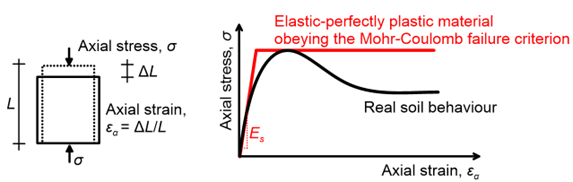
The simplest model used in practice to describe the response of soils up to failure and beyond is the elastic-perfectly plastic model obeying the Mohr-Coulomb failure criterion, referred to in the following as the Mohr-Coulomb model for brevity. The Mohr-Coulomb model is used to describe the real soil stress-strain response under different stress paths e.g., unconfined uniaxial compressive (UC) loading (Figure 5.1a) with an idealised elastic-perfectly plastic stress strain curve (Figure 5.1b), that is straightforward to define as it requires the minimum number of input soil parameters.

(a) (b)

The figure on the left presents a schematic of an unconfined compression test. The axial stress is σ and the axial strain is εα=ΔL/L where L is the heigh of the sample and ΔL is the axial compression of the sample. The figure on the right presents idealised measurement from that test, in the form of axial stress-axial strain curve. The softening behaviour of the real soil is approximated by a bilinear curve, representing the elastic-perfectly plastic material model obeying the Mohr-Coulomb failure criterion. — Figure 5.1. (a) Schematic of an unconfined compression test (b) Strain-strain curve.

It is reminded here that the stress state of any soil element can be described with Mohr’s circle, depicted in Figure 5.2 for two-dimensional conditions.

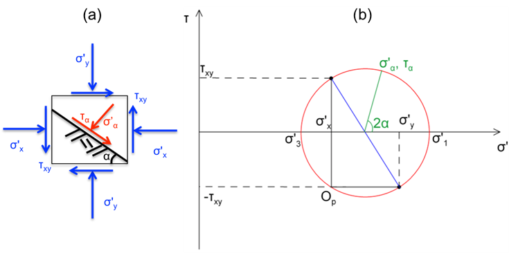
Figure (a) on the left presents a 2D soil element, with normal effective and shear stress acting on its edges. The normal and shear stress along a plane inclined at an angle a relevant to the horizontal is also shown. Figure (b) on the right presents the Mohr's circle of stress for that element, denoting the principal stresses, as well as stresses at the plane incline at an angle a. — Figure 5.2. (a) Stress state of a soil element under general loading, and (b) the corresponding Mohr’s circle for stresses.

The Mohr-Coulomb failure criterion suggests that the following inequality 5.3 is valid for all planes passing through the soil element in Figure 5.2, with the inclination of the plane defined by angle α:

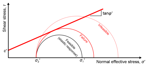
(5.3) ${\tau _\alpha } \le c' + {\sigma '_\alpha }\tan \varphi '$

As depicted in Figure 5.3, the Mohr-Coulomb failure criterion describes a line (envelope) in the σ′–τ effective normal stress-shear stress space. In effective stresses, this envelope is defined by the soil’s effective cohesion c′ and the friction angle φ′. Note that symbols φ′ and φ are often used interchangeably, and both represent friction angle under effective stress. For any given stress state applied to the soil element, the Mohr’s circle lies below the failure line (feasible area), or is tangent to it. In the first case the soil remains elastic, whereas in the second case the soil has reached failure (Figure 5.3).

Graph illustrating the Mohr-Coulomb failure criterion in the shear stress-normal effective stress space. Three Mohr's circles are plotted, a feasible one corresponding to elastic response, the Mohr's circle at failure which is tangent to the failure line, and an infeasible one that crosses the failure line. — Figure 5.3. Mohr-Coulomb failure envelope for effective stress parameters.

Figure (a) on the left presents the Mohr's circle in the shear stress-normal effective stress space, with the Mohr's circle at failure. The normal and shear stresses at the intersection of the Mohr's circle with the failure line are denoted with σ'_f and τ_f. These stresses correspond to a failure plane inclined at an angle θ relatively to the vertical. Figure (b) on the right presents a failed triaxial clay sample, with the inclined failure plane denoted with a red dashed line. — Figure 5.4. (a) Mohr-Coulomb circle at failure considering effective stress parameters (drained response) and (b) failure plane formed in an unconfined compression (UC) test.

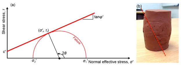
Failure of the soil element takes place at a plane defined by angle θ, where the shear stress and the normal stress acting on this plane satisfy Eq. 5.4 (Figure 5.4):

(5.4) ${\tau _f} = c' + {\sigma '_f}\tan \varphi '$

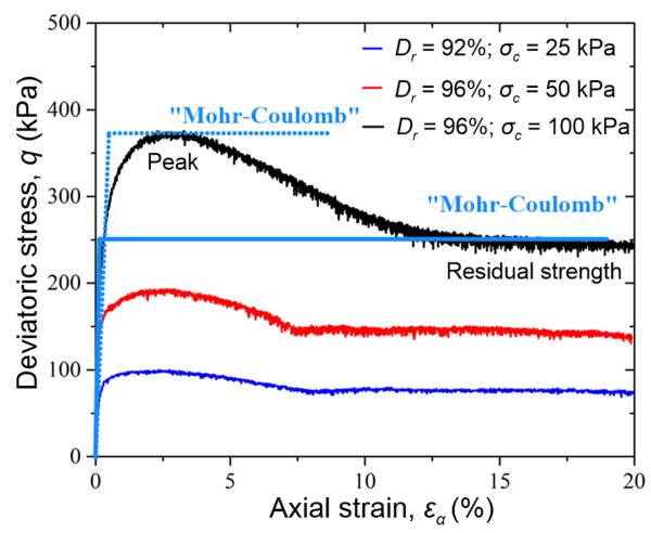
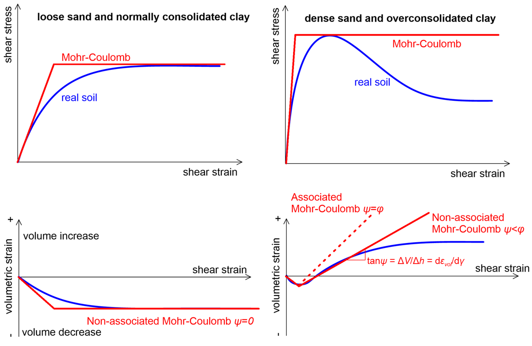
When no excess water pore pressure develops in the soil upon loading, its response is called drained, and failure can be described with the effective stress parameters c′, φ′. This type of response can be simulated in PLAXIS with the Mohr-Coulomb Drained soil model. Remember that the drained soil compressibility parameters (Young’s modulus E′, Poisson’s ratio v′) must be used to quantify its linear elastic response up to failure. Properly using the Mohr-Coulomb model, which allows describing soil strength with only two (plus the dilation angle, as we will see later) parameters, requires understanding and appreciating the deficiencies of such a simplified approach. First of all, dilating soils such as dense sands will reach a peak strength during shearing, and their strength will drop to a residual value at relatively large strains (Figure 5.5). Depending on the selection of the friction angle φ′ we can capture either the peak or the residual strength with the Mohr-Coulomb model-not both. Which one we will choose to capture depends on the nature of the problem.

Graph depicting results of three triaxial compression tests performed in dense sand (Dr = 92% to 96%), in terms of deviatoric stress-axial strain curves. The three tests correspond to confining stresses σ_c = 25, 50 and 100 kPa. All three curves indicate that the sand samples exhibited softening during shearing. Two bilinear curves are fitting to the stress-strain curve of the sample sheared under the maximum confining stress, indicating different fits of the Mohr-Coulomb model at the peak and the residual strength. — Figure 5.5. Deviatoric stress-axial strain curves obtained during the shearing stage of isotropically-consolidated (confining stress *σ_c* = 25, 50 and 100 kPa) triaxial compression tests on dense Stockton Beach sand samples.

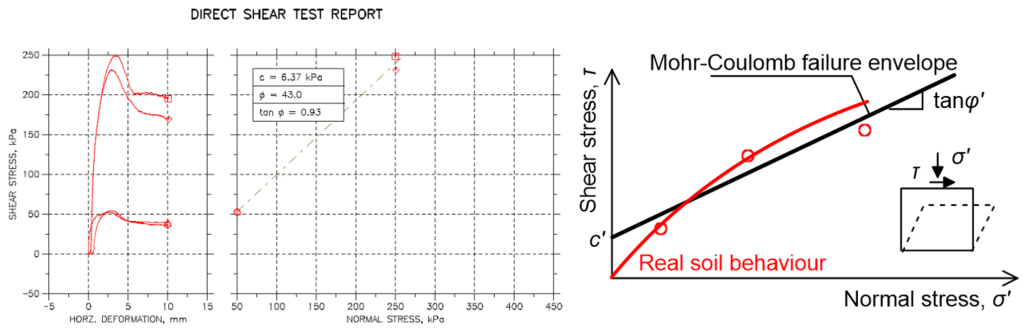
Another important simplification introduced in the Mohr-Coulomb model is that the failure envelope in the σ′–τ space is a straight line (Figure 5.3). However, the failure envelope of real soils is not linear, in other words the friction angle φ′ actually depends on the level of confining stress that the soil is being subjected to during shearing. As consequence, the Mohr-Coulomb shear strength parameters selected to estimate the collapse load must be compatible with the normal stress levels experienced by soil for the particular problem. To further delve into that, Figure 5.6a presents measurements obtained during four direct shear tests in dense dry Stockton Beach sand, a non-cemented silica sand that certainly has zero strength under zero normal stress or c′ = 0. However, linear fitting of the test data by the direct shear testing device software to automatically obtain strength parameters yielded effective cohesion c′ = 6.3 kPa. This is not an error, but a consequence of attempting to describe the sand failure envelope with two parameters (Figure 5.6b). The automatically calculated strength parameters will accurately describe Stockton Beach sand shear strength if the normal stress acting on shear planes are between 50 kPa and 250 kPa, but will result in erroneous predictions if e.g., the normal stress is significantly lower. As one would expect there exist material models (some of which implemented in PLAXIS) that incorporate non-linear failure criteria, thus are capable of quantifying soil strength across a wide range of normal stresses with a single set of parameters. However, description of such (more advanced) material models is beyond the scope of this Part.

The figures on the left are screenshots of the direct shear device software. They present shear stress versus horizontal deformation curves exhibiting softening, and fitting of the residual values in the normal stress-shear stress space to obtain the parameters of the Mohr-Coulomb failure criterion. The figure on the right shows a linear Mohr-Coulomb failure envelope at the shear stress-normal stress space, with cohesion intercept larger that zero. This figure also shows a curved non-linear failure envelope indicating real soil behaviour, where the cohesion intercept is zero and the inclination of failure envelope increases as normal stress increases. — Figure 5.6. (Left) Shear stress-horizontal deformation and fitting Mohr-Coulomb failure envelope from four (4) direct shear tests on dense Stockton Beach sand (normal stress 50 and 250 kPa); (Right) Comparison of linear Mohr-Coulomb failure envelope and real (non-linear) soil failure envelope.

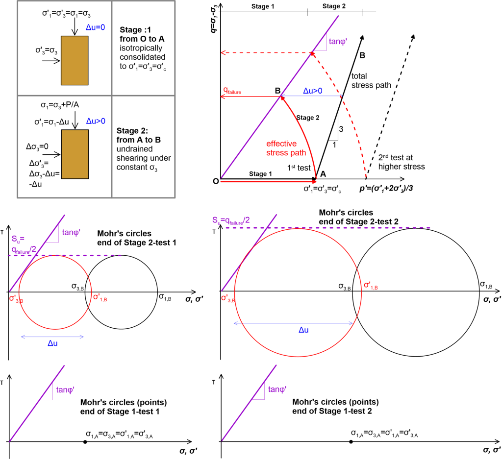
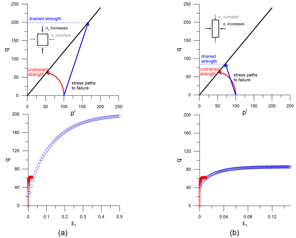
Excess pore pressure Δu may develop during and shortly after the application of external stresses on fine-grained soils exhibiting low permeability. This excess pore pressure should be accounted for the estimation of the effective normal stress acting on the failure plane. Considering explicitly the excess pore pressure that develops up to failure is not an easy task, and certainly the Mohr-Coulomb model, due to its simplicity, is not capable of providing realistic estimates. To tackle this problem, we resort to defining failure in terms of total (instead of effective) stresses. This concept is introduced in Figure 5.7 below, which presents results of two conceptual undrained triaxial tests on isotropically consolidated clay samples reconstituted from slurry (therefore normally consolidated at the end of Stage 1). During the undrained shearing Stage 2, excess pore pressure develops, and failure takes place at a deviatoric stress q less than the deviatoric stress that the sample would fail if sheared slowly enough that drained conditions would prevail, and effective stresses were equal to total stress (Δu = 0). As before, failure occurs when the effective stress circle becomes tangent to the Mohr-Coulomb failure line. In other words, soil still obeys the failure criterion defined in Eq. 5.1 and depicted in Figure 5.3.

To alleviate the need for calculating excess pore pressure, we can define failure through the Mohr’s circle of total stresses which we know, as they are the externally applied stresses on the soil sample. The failure plane for total stress is horizontal, and intersects the shear stress axis at S_u= q_failure/2 = (σ′_1,failure–σ′_3,failure)/2 = (σ_1,failure– σ_3,failure)/2. We call the deviatoric stress at failure (divided by 2), S_u the undrained shear strength of the soil sample.

Note however that the undrained shear strength is not a fundamental material parameter, as it depends on the effective (pre)consolidation stress σ′_c, and the overconsolidation ratio OCR. This is clear in Figure 5.7, where a sample of the same soil isotropically consolidated at a higher stress (test 2) and thus featuring a lower void ratio (water content), fails under higher deviatoric stress, therefore will have a higher undrained strength.

The figure on the top left presents two stages of an isotropically consolidated undrained triaxial test. Stage 1 from O to A is the isotropic consolidation stage, and Stage 2 from A to B is the undrained shearing stage. The figure on the top right presents results of two triaxial tests, performed at different confining stress. at the p'-q space. Both the effective and total stress paths are shown, and the excess pore pressure is indicated. Stress paths from both tests terminate at the critical state line. The figures at the bottom present Mohr's circles at the end of stage 1 and at the end of stage 2, for two triaxial tests performed at different confining stress. Both total and effective Mohr's circles are plotted. — Figure 5.7. Schematic of isotropically consolidated undrained triaxial tests (CU) in two clay samples.

Some readers may erroneously associate the terms drained and undrained tests or soil behaviour with the presence of groundwater table, or even just drainage boundary conditions. However, the terms drained and undrained in soil mechanics context refer to the development or not of excess pore pressures in soil upon its loading, in situ or in the laboratory. Whether a soil will behave as drained or undrained in situ depends on its permeability and the rate of loading. It is reminded that soils above the groundwater table may still be saturated, and will develop excess pore pressures (will behave as undrained) after the application of an external loading, if their permeability is low. Bishop and Eldin (1950), who were among the first to use the terms undrained and drained, explain that undrained tests were referred to prior to 1949 as “immediate tests” in England and “quick tests” in the USA, Netherlands and Belgium since, owing to the low permeability of clay soils, the same result is obtained if the test is performed relatively quickly, even if drainage is not prevented during laboratory soil testing, because excess pore pressures cannot dissipate fast enough. Similarly, drained tests were referred to as “slow tests”, since slow testing rate was required to ensure full dissipation of excess pore pressures, even when drainage is not prevented. However, the terms slow and fast can be misleading when dealing with soils of different permeabilities, and are not used anymore: For example an undrained test in clay may require several months to complete, while a drained test in sand may be completed in minutes.

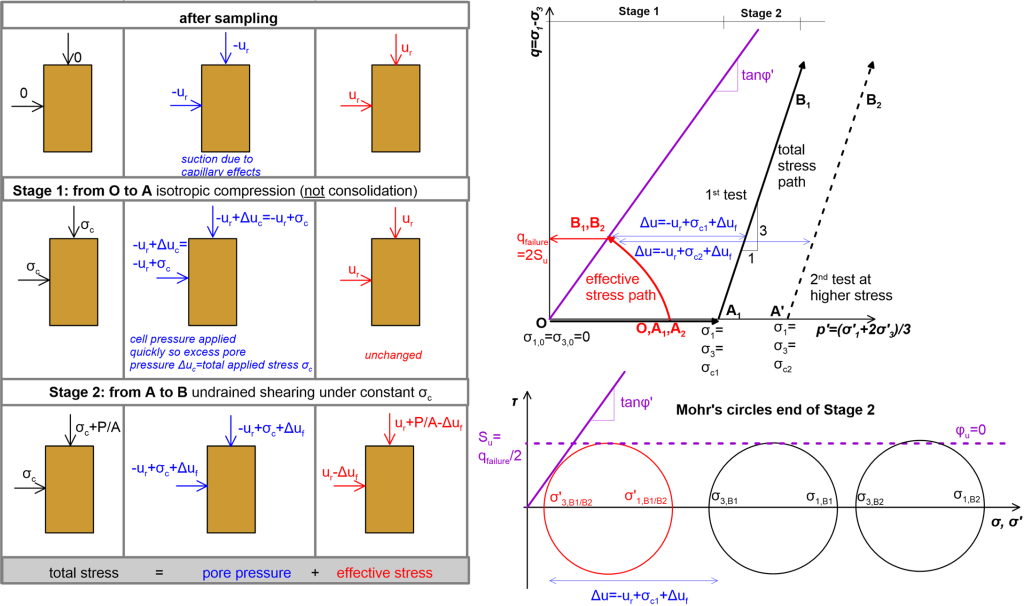
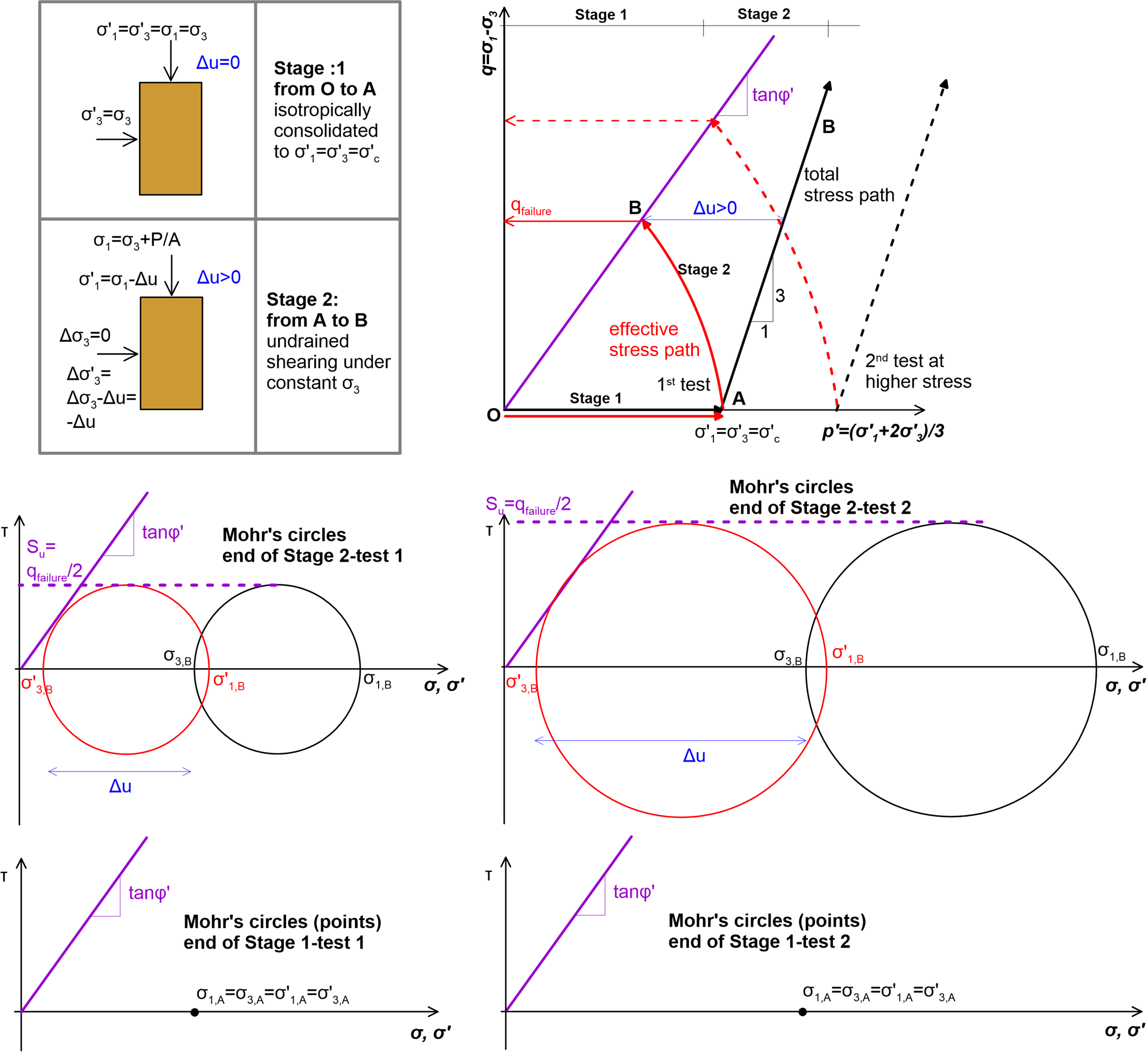
There is a common misconception that the undrained shear strength does not depend on the level of stresses and is a material constant, which has its origins in the use of unconsolidated undrained triaxial tests to quickly (as these tests are fast) determine the shear strength of samples in the laboratory. Indeed, when the sample is compressed quickly and is not allowed to consolidate (Figure 5.8) the effective stresses at the beginning of the shearing stage will remain the same, regardless of the level of applied confining (total) stress. Therefore, samples compressed at different levels of confining stress will fail at the same deviatoric stress as they will follow the same effective (but not total) stress path, hence exhibit the same undrained strength. In other words, Mohr circles under different total stress levels may be different, but the corresponding circles for effective stresses are all the same, and tangent to the effective stress failure envelope (Figure 5.8). This observation though is valid for unconsolidated undrained tests only. Note that an unconfined compression (UC) test that is performed under σ_c= 0 would result in the same undrained strength, and the soil sample would follow again the same effective stress path, despite total stresses being equal to zero. That is because the effective stresses are not zero, as they equilibrate the negative excess pore pressure –u_r in the sample that develops due to capillary effects. This is the reason why a clay sample retrieved from a borehole appears to have “some strength” (and is often described as “cohesive”, a term that has been avoided on purpose here) despite the total confining stress being equal to zero, and not because the soil has real cohesion due to cementation or natural fabric. The Mohr-Coulomb failure plane for total stresses is again horizontal (undrained friction angle φ_u= 0).

The figure on the left presents total stresses, pore pressure and effective stresses acting on a soil sample after sampling, during undrained isotropic compression (not consolidation), and during undrained shearing (unconsolidated undrained UU triaxial test). The figure on the top right presents results of two UU triaxial tests performed at different confining stresses in the p'-q space. The total stress paths of the two tests are different, but the effective stress paths are the same and end at the critical state line. The figure at the bottom right presents the Mohr's circles from the shearing stage of these two tests, and it is shown that while the Mohr's circles of total stresses are different, the Mohr's circles of effective stresses coincide. — Figure 5.8. Schematic of unconsolidated undrained triaxial tests (UU) in two clay samples.

Some fundamental conclusions arise from this discussion, which are particularly important for modelling of failure of soils under undrained conditions:

Soil fails under exactly the same “frictional sliding” mechanism, regardless of whether it is sheared under drained or undrained conditions.
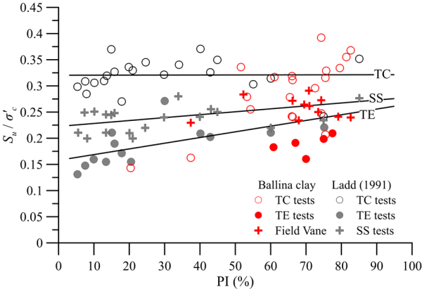
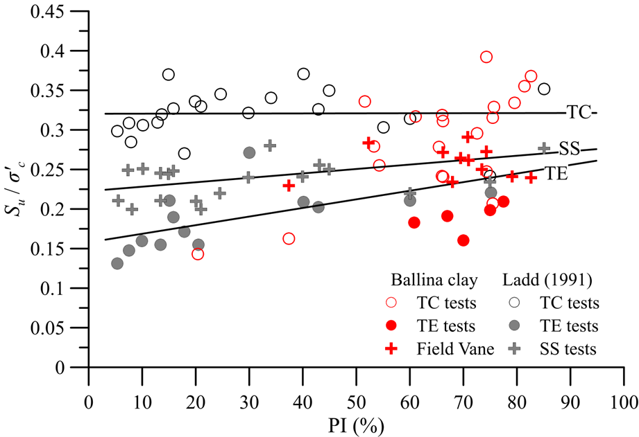
The undrained shear strength depends on the preconsolidation stress of soil, and is not a material parameter. The preconsolidation stress will increase with depth (as geostatic stresses increase), therefore the undrained strength will increase with depth even in uniform, normally consolidated soil. For a normally consolidated soil under geostatic stress S_u/σ′_z0≈ 0.22 or generally S_u/σ′_c≈ 0.22 where σ′_c is the preconsolidation stress. This is in line with Eq. 5.3 which suggests that the same soil will exhibit higher strength if found under higher confining normal stress.
The undrained shear strength must be used to define failure together with total stresses only (total stress analysis). This response is simulated in PLAXIS with the Mohr-Coulomb Undrained (C) The undrained soil compressibility parameters (Young’s modulus E_u, Poisson’s ratio v_u) must be considered together with this model to describe linear elastic response up to failure, and the undrained shear strength S_u obtained from tests is provided as a model parameter. Certainly PLAXIS, as well as most geotechnical Finite Element Codes, allows considering a linear increase of undrained strength with depth along a particular soil layer by defining S_u,inc(units: stress/unit depth) thus satisfying the described mechanisms.

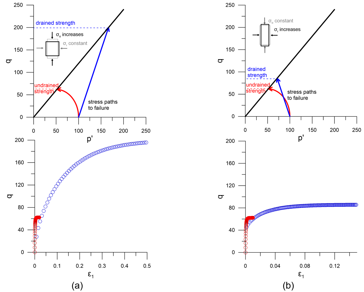
It is perhaps clear from the above that soil strength (and the collapse load of foundations on it) depends on the loading conditions: drained or undrained. However, it also depends on the stress path that is followed to failure, as depicted in Figures 5.9 and 5.10. The stress path to failure is the field is rarely known (Figure 5.11) and therefore it is common to consider an average (or mobilised) shear strength.

Figure (a) on the left presents results of idealised drained and undrained isotropic triaxial compression tests on normally consolidated soil, in the p'-q space (top) and in the q-ε1 space (bottom). The undrained strength in compression is much lower than the drained strength in compression. Figure (b) on the right presents results of idealised drained and undrained isotropic triaxial extension tests on normally consolidated soil, in the p'-q space (top) and in the q-ε1 space (bottom). The undrained strength in extension is similar to the drained strength in extension. — Figure 5.9. Simulated isotropically consolidated drained and undrained triaxial tests (CU) in (a) triaxial compression and (b) triaxial extension. Normally consolidated clay (OCR=1).

Variation of the undrained strength ratio Su/σ'c with the plasticity index of different clays (Ballina clay and data from Ladd 1991). It is shown that the undrained strength ratio depends on the stress path to failure (TC, SS, TE). TC tests provide consistently the higher strength and TE provide consistently the lowest strength. — Figure 5.10. Undrained shear strength normalised against the preconsolidation stress from triaxial compression (TC), triaxial extension (TE), simple shear (SS) and field vane tests. Results from different clays around the world and Australia (Ballina clay) (Kouretzis et al. 2017).

Schematic of a circular failure surface developing during failure of a fill. It is shown that the stress paths followed by soil elements along that failure surface vary, and range from triaxial compression near the crest to simple shear at the bottom and triaxial extension near the outcropping failure surface. — Figure 5.11. Stress paths to failure underneath an embankment.

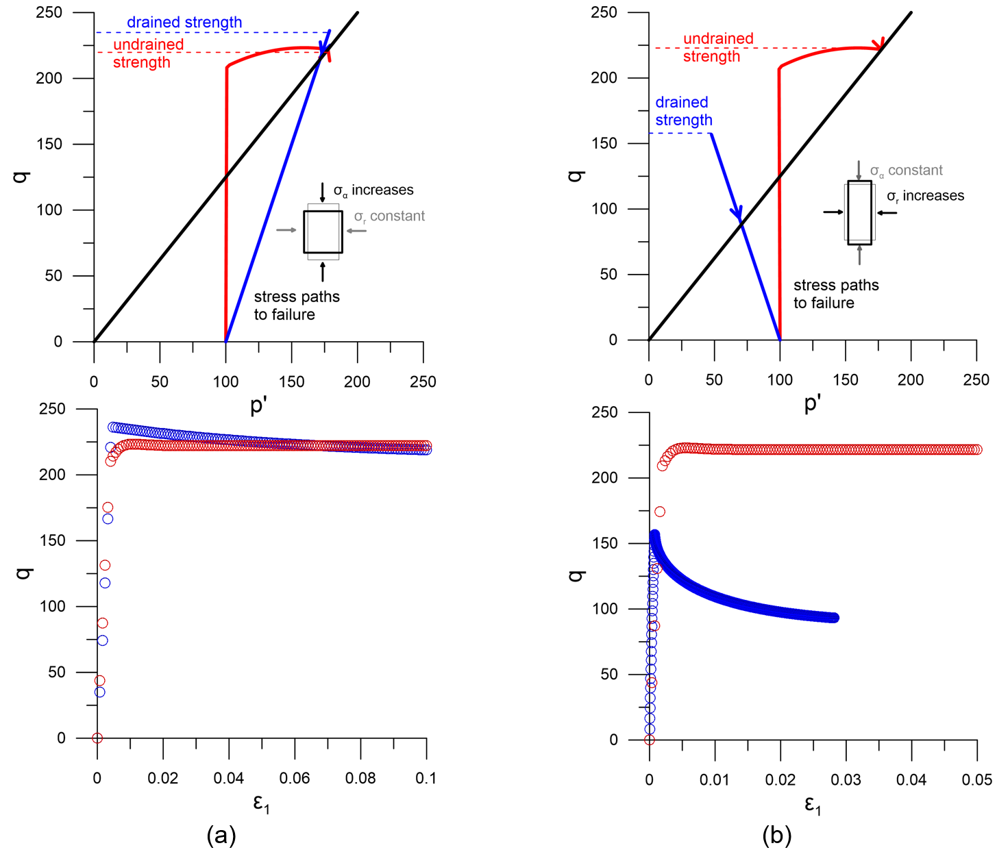
On a similar note, Figures 5.7 to 5.9 all suggest that the shear strength under undrained loading conditions is consistently lower than the strength that the same soil will exhibit under drained conditions. This is true for contracting soils that develop positive excess pore pressures upon loading, such as normally or lightly-overconsolidated soft clays. However, this is not the case for soils exhibiting dilative response, such as overconsolidated clays, which will develop negative pore pressures (suction) when sheared under undrained conditions. This will result in their undrained strength being higher than the drained strength, as depicted in Figure 5.12 and described mathematically again by Eq. 5.3. In cases like these, both the short-term (undrained) and long-term (drained) collapse load must be calculated to identify the critical load case, as discussed in the following.

Figure (a) on the left presents results of idealised drained and undrained isotropic triaxial compression tests on overconsolidated soil, in the p'-q space (top) and in the q-ε1 space (bottom). The undrained strength in compression is similar to the drained strength in compression. Figure (b) on the right presents results of idealised drained and undrained isotropic triaxial extension tests on overconsolidated soil, in the p'-q space (top) and in the q-ε1 space (bottom). The undrained strength in extension is considerably higher than the drained strength in extension. — Figure 5.12. Simulated isotropically consolidated drained and undrained triaxial tests (CU) in (a) triaxial compression and (b) triaxial extension. Overconsolidated clay (OCR=5).

Finally, it is worth discussing briefly the effect of the flow rule used together with the Mohr-Coulomb Drained model on the estimation of the bearing capacity or the collapse load with numerical methods. The flow rule in the model controls the amount of volumetric deformation (volume change) that takes place at failure, via the dilation angle ψ, which depends on the level of confining stress; a dilative soil which volume tends to increase upon shearing, such as a dense sand (Figure 5.13), will behave as contractive if sheared under high confining stress. It was mentioned in Example 4.2 that consideration of non-associated flow rule (ψ ≠ φ′) will result in more realistic estimates of volumetric deformation in soils, as also depicted below in Figure 5.13. This comes at the expense of complications related to localisation, mesh-dependency of the solution and possible convergence issues. On the contrary, it is widely accepted that adoption of associated flow will generally result in overestimation of the collapse load: Overestimating volumetric soil strains will result in overpredicting the normal stress acting on shear planes (particularly for problems with increased confinement, such as embedded foundations), and therefore the shear strength according to Eq. 5.3. A technique to avoid this, while still using associated flow in the analysis model by setting ψ = φ′ is to numerically estimate the collapse load while using an equivalent friction angle φ* = ψ* and effective cohesion c* calculated as (Davis, 1968):

(5.5) $\tan {\varphi ^ * } = n\tan \varphi '$

(5.6) ${c^ * } = nc'$

(5.7) where $n = \dfrac{{\cos \varphi '\cos \psi }}{{1 - \sin \varphi '\sin \psi }}$

Keep also in mind that when using the Mohr-Coulomb Undrained (C) soil model we impose an associative flow rule, as ψ = φ_u= 0 ensures that no volume change takes place during undrained loading (Figure 5.13).

The figure on the top left presents fitting the hardening shear stress-shear strain behaviour of loose sand and normally consolidated clay with a bilinear Mohr-Coulomb model. The figure at the bottom left presents fitting the contracting volumetric strain-shear strain behaviour of loose sand and normally consolidated clay with a bilinear non-associated Mohr-Coulomb model. The figure on the top right presents fitting the softening shear stress-shear strain behaviour of dense sand and overconsolidated clay with a bilinear Mohr-Coulomb model. The figure at the bottom right presents fitting the dilating volumetric strain-shear strain behaviour of dense sand and overconsolidated clay with a bilinear non-associated Mohr-Coulomb model. — Figure 5.13. Soil behaviour and associated/non-associated Mohr-Coulomb models.

Summarising:

When excess water pore pressures do not develop upon loading of the soil, or have already dissipated (drained loading), as it will be the case for:

Dry soils.
Coarse-grained soils (sand, gravel) with high permeability.
Saturated fine-grained soils (clay, silt) with low permeability, when we are interested in their long-term behavior e.g., long-term stability of an excavation or an embankment, after dissipation of excess pore pressures that developed during construction.

use the Drained Mohr-Coulomb model with effective shear strength and compressibility parameters (E′, v′, c′, φ′, ψ). If the Mohr-Coulomb model is used together with an associate flow rule (ψ = φ′) to obtain the collapse load, it is recommended to use equivalent shear strength parameters from Eqs. 5.5-5.7.

When excess water pore pressure may develop upon loading of the soil (undrained loading), as it will be the case of:

Saturated fine-grained soils (clay, silt) with low permeability, when we are interested in their short-term behavior e.g., collapse of a footing during and immediately after construction, or under dynamic loads; stability of an embankment during fill works, and immediately after construction.

use the Undrained (C) Mohr-Coulomb model with total shear strength and compressibility parameters (E_u, v_u≈0.5, S_u). The considered S_u value needs to properly account for the preconsolidation stress and of the overconsolidation ratio, as these cannot be computed automatically by PLAXIS with the particular soil model.

Note that for simplicity in the following examples we will consider generally the undrained shear strength to be constant, in line with the assumptions of most simple analytical solutions. However, the reader must understand that this by no means suggests that considering an appropriate undrained strength profile with depth is not required in practical problems.

License

Icon for the Creative Commons Attribution 4.0 International License

Fundamentals of foundation engineering and their applications Copyright © 2025 by University of Newcastle & G. Kouretzis is licensed under a Creative Commons Attribution 4.0 International License, except where otherwise noted.