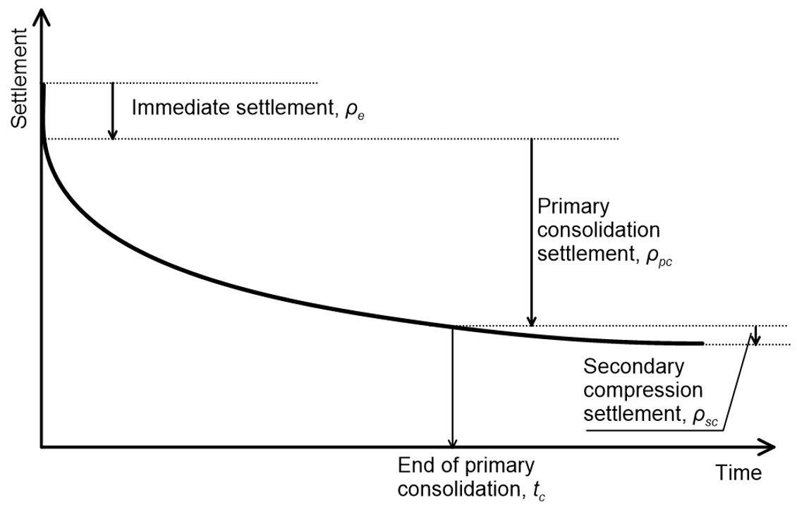
4.8 Evolution of primary consolidation settlement with time
The rate of dissipation of excess pore water pressure, and thus the necessary time for the applied loading on the ground surface to be transferred to the soil skeleton resulting in increase of the effective stress, depends on the permeability, k of the soil. We can obtain a closed-form analytical expression that provides the rate of dissipation of excess pore pressure, and thus the evolution of settlement with time (Figure 4.7), under some simple assumptions:
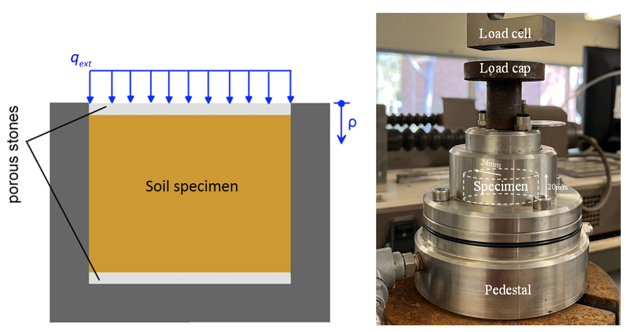
- 1-D conditions prevail, with water flowing only vertically, as in the oedometer test (Figure 4.27).
- The soil is fully saturated, homogeneous and isotropic.
- Darcy’s law is valid, thus flow q is equal to the permeability times the hydraulic gradient i i.e., q=ki
- Small strains.
Under the above assumptions, Terzaghi formulated the one-dimensional consolidation equation, describing the variation of excess pore pressure u with time t and depth z as:
(4.65) 
The constant cv in the differential equation 4.65 is called coefficient of consolidation, and depends on the coefficient of volume compressibility mv and the soil permeability in the vertical direction kz as:
(4.66) 
where γw ≈ 10 kN/m3 is the unit weight of the water. The coefficient of consolidation carries units of length2/time.
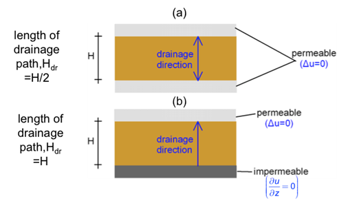
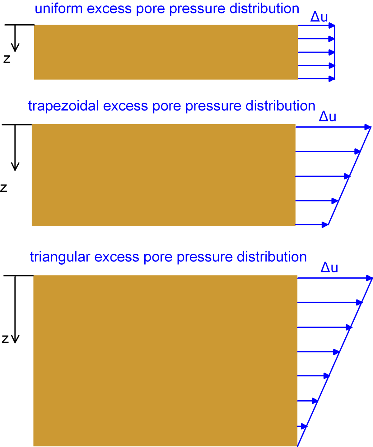
Solution of the differential equation 4.65 requires knowing the initial distribution of excess pore pressure with depth (Figure 4.38), and the permeability boundary conditions. For example, assuming uniform excess pore pressure distribution with depth, corresponding to a relatively thin clay layer (Figure 4.38) and double drainage, both from the top and the bottom of the layer (Figure 4.39a):
- at t = 0, the excess pore pressure will be uniform along the thickness, and equal to the applied pressure at the surface Δu0 = qext
- at the top boundary z=0 where drainage is allowed, Δu = 0
- at the bottom boundary z=H where drainage is allowed too, Δu = 0

The drainage boundary conditions suggest that excess pore pressure will immediately fall to zero at the permeable boundaries.
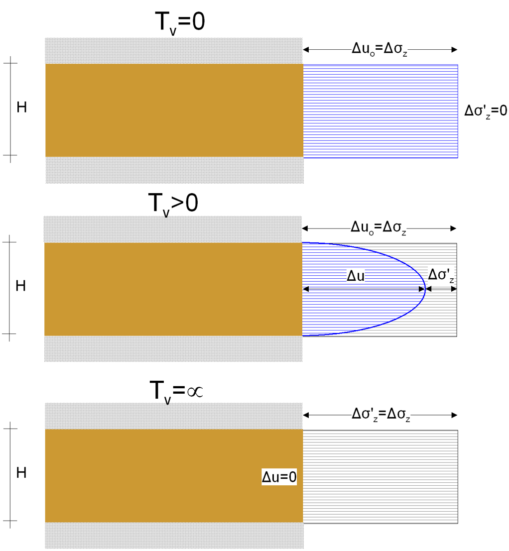
A closed-form solution of Eq. 4.65 exists for the above conditions and provides the variation of the excess pore pressure with depth at different time instances (Figure 4.40):
(4.67) 
where  , and Tv is the time factor, equal to:
(4.68) 
The length of the drainage path, Hdr depends on the drainage boundary conditions, and is depicted in Figure 4.40.
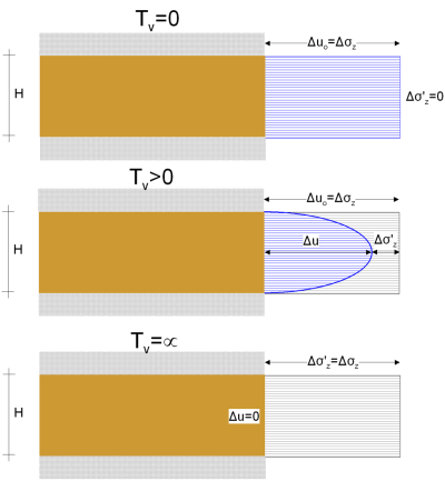
Instead of using the absolute value the of excess pore water pressure, consolidation progress can be described via the degree of consolidation (or consolidation ratio), U(z) which defines the amount of consolidation completed at a particular time instance, at a specific depth, z:
(4.69) 
The degree of consolidation is visualised as the grey shaded area in Figure 4.40. From an engineering point of view, we are rather interested in the average degree of consolidation, U of the whole compressible layer. For the special case where the initial excess pore pressure distribution is assumed constant with depth (Figure 4.38) the average degree of consolidation is calculated as:
(4.70) 
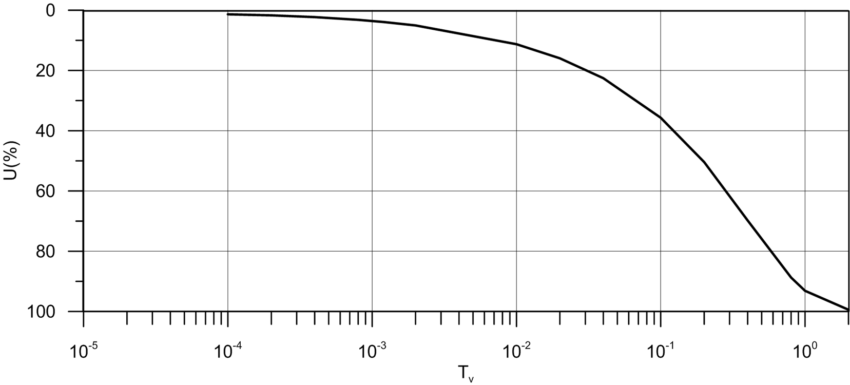
The variation of the average degree of consolidation with the time factor Tv is illustrated in Figure 4.41.
Eq. 4.70 and Figure 4.41 are also valid when drainage is not allowed at the bottom of the clay layer. The length of the drainage path in that case will be Hdr = H (Figure 4.39). Note that at an impermeable boundary, the gradient of pore pressure will be zero  = 0.
= 0.
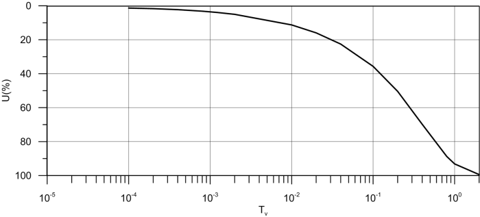
Note that Figure 4.41 can be used to estimate settlement of a 1-D soil column at any given time t1. By substituting t1 into the expression for the time factor Tv (Eq. 4.68) we can find the average degree of consolidation U1 at t1 directly from Figure 4.41. Therefore, settlement at t1 will be:
(4.71) 
where the primary consolidation settlement ρpc is calculated according to Section 4.6.2, assuming linear elastic or non-linear soil behaviour.
