4.6 Primary consolidation settlement of shallow foundations
4.6.1 General considerations
Primary consolidation settlement is usually the larger portion of the total settlement developing in structures founded in fine-grained soft soils, at least when the applied loading is a small fraction of the collapse loading. When the applied working loading is near the collapse loading, immediate settlement is also very important, but generally good engineering practice suggests that the working loading should be considerably less than the collapse loading. Generally, we are interested not only in the magnitude of the primary consolidation settlement, but also in the evolution of settlement with time. Depending on the properties of the soil, and especially on its permeability, consolidation settlement may continue evolving for years, as in the case of the famous Leaning Tower of Pisa (Figure 4.24), although the author would argue that time-dependent tilt of the Tower of Pisa involves more complex mechanisms than the ones described in this section.
The methodology that should be followed for the estimation of the consolidation settlement of shallow foundations depends on the geometry of the problem, and more specifically on the width of the foundation, B compared to the thickness of the compressible layer of saturated clay, H (Figure 4.25). Two cases are identified:

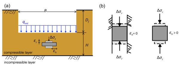
If the width of the loaded area is significantly larger than the thickness of the compressible layer B > (3 to 4)H, we can assume 1-D loading conditions i.e., the lateral strain can be taken equal to zero εx = εh = 0. Furthermore, the additional total stress due to the applied loading Δσz can be assumed practically constant with depth (see Figure 3.11 and Example 4.3), and will be equal to the applied pressure on the foundation level Δσz = qext. At the end of consolidation, when the excess pore pressures have dissipated it will be Δσ′z = qext. In the light of these assumptions, the primary consolidation settlement ρpc is estimated from 1-D consolidation theory:
(4.17) 
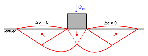
On the other hand, if the width of the loaded area is comparable to the thickness of the compressible layer B < (3 to 4)H, significant lateral strain will inevitably develop εx = εh ≠ 0 (Figure 4.25b and Figure 4.9), and loading conditions are no longer one-dimensional. As lateral strains develop, the excess pore pressure Δu immediately after the application of the external loading is lower than the 1-D case, where Δu = Δσz. On top of that, the variation of the additional stress Δσz with depth must be considered (according to Part 3) so Δσz < qext.
In view of the above, the primary consolidation settlement ρpc will be less that the settlement that would be estimated from 1-D consolidation theory:
(4.18) 
where μ < 1.0 is a factor depending on the geometry of the footing, the thickness of the compressible layer, and the properties of the soil.
Methodologies for estimating the magnitude of the primary consolidation settlement of shallow foundations for both cases mentioned above are presented in the following paragraphs, while the evolution of settlement with time is discussed in Chapter 4.8.
4.6.2 Estimation of primary consolidation settlement of shallow foundations and embankments under 1-D loading conditions
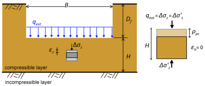
Primary consolidation settlement under 1-D conditions can be estimated either on the basis of linear consolidation theory, or using the oedometer laboratory test results. Focusing first on the former, consider a soil particle below the surface loaded with a compressive pressure qext (Figure 4.26). At t = tc, (see Chapter 4.8) when excess pore pressures will have dissipatedand the full primary consolidation settlement will have developed, the total external pressure will have been transferred to the soil skeleton, as effective stress (Figure 4.26). The volume of a soil column with unit width will have decreased from:
(4.19) 
to
(4.20) 
so the volumetric strain εvol = εx + εy + εz = εz for 1-D conditions will be equal to:
(4.21) 
where ρpc is the primary consolidation settlement, and H is the thickness of the compressive layer. The volumetric strain is related to the soil properties via the coefficient of volume compressibility (or coefficient of volume decrease) mv as:
(4.22) 
where Δσ′z is the additional effective stress due to the application of the external loading. The coefficient of volume compressibility is associated to the drained Young’s modulus and Poisson’s ratio of the soil E′, v′ as:
(4.23) 
For the common case of v′ = 0.333 it is mv = 2/(3E′). Substituting now Eq. 4.22 into Eq. 4.21 yields the expression for estimating consolidation settlement assuming linear elastic response of the soil, as:
(4.24) 
The main drawback of this approach is that, in reality, the coefficient of volume compressibility mv is not constant, but depends on the stress level (as E′ does). This suggests that we must select an mv value compatible with the expected stress level.
It is worth noting here that Eq. 4.24 can be used together with Eq. 4.23 to calculate total settlement of coarse-grained soils too, when subjected to 1-D loading conditions. It is based on the theory of elasticity, hence it is applicable to any material that can be assumed to behave as elastic. At the end of consolidation, when excess pore pressures have completely dissipated, both fine grained and coarse grained soils will behave as drained, therefore the same linear elastic formulas can be used to estimate their deformations.
Methods for calculating consolidation settlement of fine-grained soils provide reasonably accurate results, if the stress applied in soil does not result in soil yielding i.e., the final vertical effective stress of soil does not exceed its preconsolidation stress σ′c which, for vertical loading, is the maximum vertical stress that the soil has undergone in the past σ′zc. If this is not the case, then selecting an appropriate mv value is cumbersome, because mv increases rapidly as the applied stress in soil exceeds σ′c.
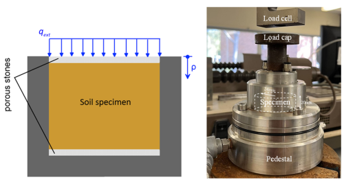
Alternatively, 1-D consolidation settlement can be estimated on the basis of laboratory test results, considering explicitly non-linear soil response. In that case we do not have to select an appropriate stress level to “calibrate” soil stiffness. The phenomenon of consolidation can be replicated in the laboratory with the oedometer device: an undisturbed soil specimen is placed in a cylindrical mold, with porous stones positioned on the top and at the bottom of the sample, to allow drainage (Figure 4.27). The mold is rigid, and no lateral strains are allowed to develop, therefore ensuring 1-D conditions. A load is applied on the top of the specimen, and the variation of the void ratio of the soil with applied pressure and time is measured.
It is reminded that the void ratio, e is equal to the volume of the voids over the volume of solids of the soil specimen:
(4.25) 
and the initial specific volume of the soil sample is v = 1+e0, with e0 being the initial void ratio. Keeping in mind that changes in the soil volume are due to changes in the volume of voids only, the volumetric strain is written as:
(4.26) 
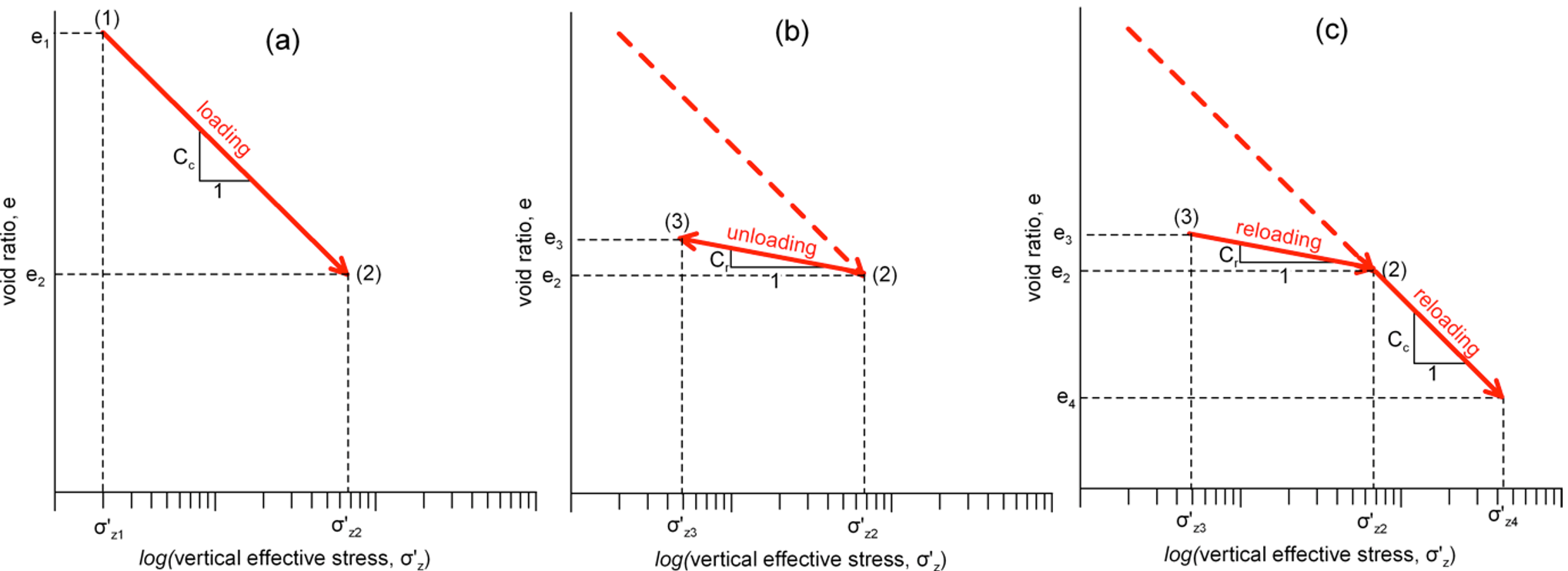
The minus sign in Eq. 4.26 suggests that positive volumetric strains are compressive. Results of the oedometer test are usually plotted in e-logσ′z graphs, as shown in Figure 4.28. From the initial loading stage, where the effective stress increases from σ′z1 to σ′z2 (Figure 4.28a), we can define the slope of the normal consolidation line NCL [path (1)-(2), Figure 4.29]:
(4.27) 
The slope of the normal consolidation line Cc in the e-logσ′z space is called compression index. If we unload the sample from effective stress σ′z2 to a lower effective stress σ′z3, the soil will not follow the initial loading line, but rather the unloading-reloading line URL [path (2)-(3), Figure 4.29] in Figure 4.28b. The slope of this line Cr called recompression index
(4.28) 
will be lower than the slope of the normal consolidation line, due to the fact that soil is actually a non-linear material, and application of the stress σ′z2 resulted in irreversible changes in the soil fabric. In the hypothetical case where the soil behaved elastically, the recompression index would be equal to the compression index Cc = Cr. If we reload the soil from stress σ′z3, it will follow the unloading-reloading line [path (3)-(2)] until it reaches the maximum vertical effective stress applied previously, σ′z2. The void ratio variation along the path (3)-(2), and thus the increase in vertical deformation (settlement), will be relatively small, because the soil fabric has been permanently changed in the past.
However, if the soil is further subjected to stresses higher than the past maximum vertical effective stress σ′z2, along the path (3)-(2)-(4) in Figure 4.29, the settlement for the stress increase along the path (2)-(4) will be higher for the same stress increase, compared to the path (3)-(2), as the soil will now undergo further fabric change. The slope of the path (2)-(4) is equal to the slope of the path (1)-(2) i.e., equal to the compression index.
If the maximum vertical stress that the soil has undergone in the past is σ′zc (referred to as yield stress or preconsolidation stress, as explained earlier) and its geostatic (current) vertical effective stress is σ′z0 we can define the overconsolidation ratio OCR as:
(4.29) 
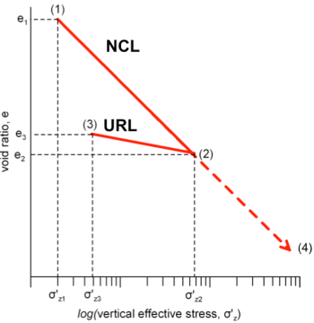
Soils with OCR > 1 are called “overconsolidated”, and will follow a path similar to (3)-(2)-(4) when loaded. Soils with OCR = 1 are called “normally consolidated”, and will follow a path similar to (1)-(2)-(4) upon loading. It must be noted here that natural soils on which onshore structures are founded rarely, if ever, feature OCR = 1. That is because fluctuation of water table levels over the geological history of a soil deposit will result in variation of effective soil stress, thus introduce some overconsolidation. Therefore even soft clays will generally have OCR > 1.1-1.2. This does not apply to soil samples that are reconstituted in the laboratory, for with OCR will be equal to OCR = 1. On a similar note, OCR cannot be less than 1 in the field, unless during soil deposition, when excess pore pressures may exist. However, this is mainly of theoretical interest.
Using the results obtained from oedometer tests in undisturbed soil specimens i.e., the values of the compression and the recompression index, the initial void ratio and the preconsolidation stress (or OCR), we can estimate the primary consolidation settlement of both normally consolidated and overconsolidated soils. Assume that the initial e.g., geostatic vertical effective stress is equal to σ′z0, and an external loading is applied, increasing the effective stress after dissipation of excess pore water pressure by Δσz to:
(4.30) 
Consolidation settlement will be again equal to the product of the volumetric strain time the thickness of the compressible layer:
(4.31) 
In the case of a normally consolidated soil (Figure 4.30) the volumetric strain will be:
(4.32) 
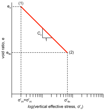
And, from Figure 4.30, the compression index will be:
(4.33) 
Combining Eqs. 4.31 to 4.33 provides the primary consolidation settlement as:
(4.34) 
Observe in Figure 4.30 that the compression index Cc, unlike the coefficient of volume compressibility mv, does not depend on the stress level (at least for soils without a natural structure). As mentioned above, when using linear theory to estimate consolidation settlement, the coefficient of compressibility mv should be estimated while considering an average value of E′ corresponding to stress levels between σ′z0 and σ′fin (see also Figure 4.14b).
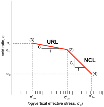
In the case of an overconsolidated soil, pre-consolidated at vertical stress σ′zc (Figure 4.31), we have to distinguish two different subcases:
If the final stress is lower than preconsolidation stress σ′fin < σ′zc, then the soil will follow the URL in Figure 4.31, and the settlement will be:
(4.35) 
In the case however where the final vertical stress is higher than the preconsolidation stress σ′fin > σ′zc, then the soil will follow initially the URL, until the applied stress reaches σ′zc, and accordingly the NCL, along the path (2)-(4) (Figure 4.31). The settlement in that case will be:
(4.36) ![{\rho _{pc}} = \dfrac{H}{{1 + {e_0}}}\left[ {{C_r}\log \dfrac{{{{\sigma '}_{zc}}}}{{{{\sigma '}_{z0}}}} + {C_c}\log \dfrac{{{{\sigma '}_{fin}}}}{{{{\sigma '}_{zc}}}}} \right]](https://oercollective.caul.edu.au/app/uploads/quicklatex/quicklatex.com-03fe4627dc08aa117dba6b3947be9504_l3.png "Rendered by QuickLaTeX.com")
4.6.3 Primary consolidation settlement of shallow foundations under 3-D loading conditions.
Skempton and Bjerrum (1957) proposed a method to modify the one-dimensional consolidation Eq. 4.24 by introducing the factor μSB, to account for the development of lateral strains below footings of finite dimensions:
(4.37) 
or, if we divide the compressible layer into n sublayers with thickness Hi :
(4.38) 
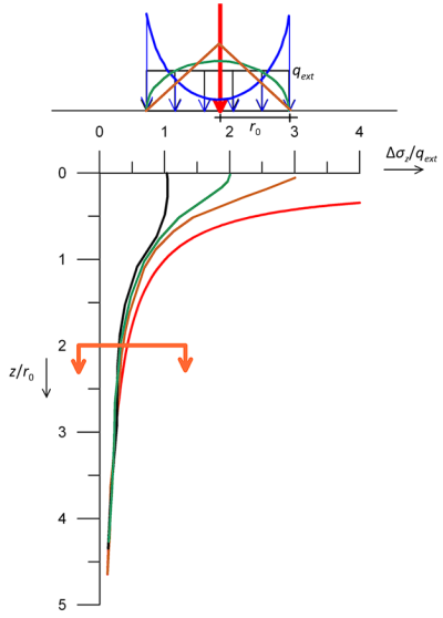
Values of μSB can be estimated from Figure 4.32, depending on the geometry of the footing, the thickness of the compressive layer H, and Skempton’s pore water coefficient A at failure, calculated as Δu = B[Δσ3+Α(Δσ1-Δσ3)] during triaxial undrained stress. As B = 1 for fully saturated samples, essentially A provides the excess pore pressure Δu that develops during the shearing stage of a triaxial test while applying a deviatoric stress (Δσ1-Δσ3). A is not constant during the test, and at failure it ranges from A = 0.5 to A = 1.0 for normally consolidated clays, and from A = 0 to A = 0.5 for stiff-to-hard overconsolidated clays. For linear elastic soil material it is A = 1/3. Thus while Eq. 4.37 resembles Eq. 4.24 used above to estimate consolidation settlement of linear elastic soil, the factor μSB actually accounts for non-linear soil behaviour via the coefficient A. For intermediate values of the thickness-to-width ratio H/B, linear interpolation can be used. Figure 4.32 is also applicable to square or rectangle footings, by considering an equivalent circular footing of diameter:
(4.39) 
where Af is the area of the square or the rectangle.
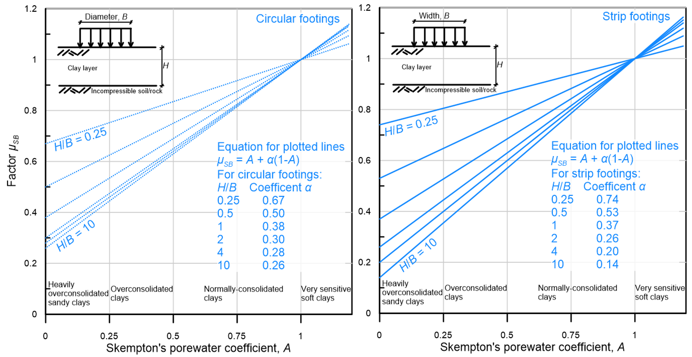
The above method provides only the settlement below the center of a footing. Finally, it is worth stressing out that this method provides settlement at the end of consolidation i.e., immediate settlement calculated according to Section 4.5.5 should be added to consolidation settlement calculated by means of Eq. 4.38.
